4 Asymptotic analysis of stochastic gradient algorithms
Consider the following stochastic gradient algorithm for solving \(\theta^* = \argmin_{\theta \in \Theta} f(\theta)\), given noisy sample access to \(f\):
\[ \begin{align*} \theta_{n+1} = \theta_n - a(n) \widehat \nabla f(\theta_n), n\ge 0. \tag{4.1} \end{align*} \]
In Chapter 3, we learned how to form \(\widehat \nabla f(\theta_n)\) from function samples so that \(\widehat \nabla f(\theta_n) \approx \nabla f(\theta_n)\). Recall that these estimators incorporate search directions based on randomly perturbed parameters. The question of the error in the simultaneous perturbation-based estimate was also handled in the earlier chapter. In this chapter, we shall be concerned with whether \(\theta_n\) governed by (4.1) converges to a local optimum \(\theta^*\) or a neighborhood of it, when the underlying gradient estimates are biased. The update in (4.1) is equivalent to
\[ \begin{align*} \theta_{n+1} = \theta_n - a(n)\bigg(\nabla f(\theta_n) + \beta_n + \eta_n \bigg), \tag{4.2} \end{align*} \]
where \(\eta_n = \widehat\nabla f(\theta_n) - \E\left[\widehat\nabla f(\theta_n) \mid \F_n\right]\) is a martingale difference term, and \(\beta_n = \E\left[\widehat\nabla f(\theta_n) \mid \F_n\right] - \nabla f(\theta_n)\) is the error in the gradient estimate. Recall that the latter is of the order \(O(\delta^2\)).
We analyse both cases of direct gradient measurements where information on sample performance (noisy though unbiased) gradients is available and zeroth order methods where one has access to only noisy function observations and not sample performance gradients. In the second case, we further consider the following sub-cases: (i) where the sensitivity parameter \(\delta\equiv\delta_n\downarrow 0\) as \(n\uparrow\infty\) and (ii) where the parameter \(\delta>0\) is held fixed in the algorithms. In the sub-case (ii), one can argue that there exists \(\epsilon >0\) such that \(\beta_n \in \overline{B}_\epsilon(0)\) (the closed ball of radius \(\epsilon\) centred at the origin) for all \(n\geq 0\). In the above, \(\F_n\) keeps a record of observations until time \(n\). For instance, in the case of SPSA, one may let \(\F_n=\sigma(\theta_m, m\le n, \Delta_m, m<n), n\ge 1\), and \(\F_0=\sigma(\theta_0)\) as the sequence of sigma algebras generated by the associated quantities. This choice of \(\F_n\) would ensure \(\Delta_n\) is independent of \(\F_n\), for all \(n\).
Map of the results
Table 4.1 provides a summary of the main convergence results for the stochastic gradient algorithm 4.1 with gradient estimates constructed using measurements from a zeroth-order oracle. The analysis of the previous chapter can be encapsulated into a biased gradient oracle, as illustrated in Figure 4.1.
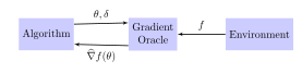
Figure 4.1: The interaction of the algorithms with a stochastic zeroth-order oracle that provides a gradient at the input point \(\theta\), with perturbation constant \(\delta\).
For a given input parameter \(\theta\) and perturbation constant \(\delta\), one could use the schemes outlined in the previous chapter to obtain a gradient estimate \(\widehat\nabla f(\theta)\) that satisfies
\[ \begin{align*} \norm{ \EE{\widehat\nabla f(\theta)} \!-\! \nabla f(\theta) } \le C_1\delta^2, \textrm { and } \EE{\norm{ \widehat\nabla f(\theta) - \EE{\widehat\nabla f(\theta)} }^2} \le \frac{C_2}{\delta^2}, \tag{4.3} \end{align*} \]
for given \(\theta\) and some constants \(C_1\) and \(C_2\).
As mentioned before, we consider both (a) the case when noisy gradient-based though unbiased estimates are available and (b) the gradient-free case where only noisy function measurements are available. In the second case (i.e., case (b)), we further consider two sub-cases for analysis. First, the gradient estimates at the \(n\)th update in (4.1) are obtained with input parameter \(\theta_n\) and perturbation constant \(\delta_n\). The sequence \(\{\delta_n\}\) is assumed to vanish asymptotically. Even though there is bias in the gradient estimates in this setting, the same asymptotically vanishes, as a result of which this setting allows analysis using the ODE approach for stochastic approximation. The unbiased (gradient-based) setting as well as the first case in the second setting (of asymptotically vanishing bias terms) form the content of Section 4.1.
The second sub-case above pertaining to zeroth-order gradient estimation, where the bias terms do not asymptotically vanish because the \(\delta\)-parameter is kept constant requires a separate, more-detailed, analysis. Here, in the \(n\)th iteration of the stochastic gradient algorithm (4.1), the input parameter considered is \(\theta_n\) while the perturbation parameter \(\delta_n\equiv\delta>0\) is a constant (i.e., is iteration-invariant). The analysis in this setting (with a constant \(\delta\)) requires more sophisticated arguments as compared to the vanishing \(\delta\equiv \delta_n\) case, and involves the theory of differential inclusions (DIs). Section 4.2 provides the DI analysis. Note that these algorithms are gradient-based algorithms where convergence can typically be claimed only to stationary points. In Section 7.2, however, we review work and provide some sufficient conditions under which one can avoid saddle points that form unstable equilibria of the associated ODE.
While this chapter focuses on the asymptotic convergence analysis, in the next chapter, we provide non-asymptotic bounds for the iterate sequence governed by (4.1).
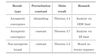
Table 4.1: Summary of the convergence results for the algorithm governed by (4.1)
4.1 Asymptotic convergence: An ODE approach
In this section, we analyse the asymptotic convergence of the algorithm (4.1) for two specific cases: (i) when direct (noisy and unbiased) gradient estimates are available, and (ii) when direct gradient estimates are not available but instead one has access to an oracle from where noisy objective function measurements at randomly perturbed parameter updates can be obtained and biased gradient estimates constructed from these. For the latter case, we assume however, in this section, that the sensitivity parameter \(\delta\) is diminishing. In other words, \(\delta\equiv \delta_n\downarrow 0\) as \(n\rightarrow\infty\), as a result of which we also show that the bias terms asymptotically vanish. This section thus treats the cases when either unbiased gradient estimates or gradient estimates that become asymptotically unbiased are available.
4.1.1 A variant of Kushner-Clark lemma for gradient systems
In this section, we provide a convergence result for a stochastic gradient algorithm with possibly biased gradient estimates. We apply this result to prove Theorem 4.4 for the case when unbiased gradient information is available. Subsequently, we analyze the stochastic gradient algorithm with biased gradient information, and use the aforementioned result in the latter setting to establish asymptotic convergence.
Consider a general stochastic gradient scheme as described in (1.3), involving the update rule below and under assumptions A2.1–A2.5.
\[ \theta_{n+1} = \theta_n + a(n) (-\nabla f(\theta_n) + \beta_n + \eta_n). \tag{4.4} \]
The ODE associated with this scheme would be
\[ \dot{\theta} = h(\theta) = -\nabla f(\theta). \tag{4.5} \]
For this ODE, \(V(\theta)=f(\theta)\) serves as a Lyapunov function. Further, \(\nabla V(\theta)^Th(\theta) \leq 0, \forall \theta\). One may now apply Lasalle’s invariance principle, see Theorem A.7–Lemma A.9 to obtain the following:
Lemma 4.1.
Any trajectory \(\theta(\cdot)\) of (4.5) must converge to the largest invariant set that is a subset of \(H \stackrel{\triangle}{=}\{\theta\mid \nabla f(\theta)=0\}\)
In the setting of gradient-based algorithms such as (1.3), we now have the following result that is easily obtained by combining Theorem 2.3 and Lemma 4.1.
In the case when the equilibrium points contained in \(\bar{H}\) are isolated, we have the following result, see Corollary 3.3 of (Benaïm 1996).
Corollary 4.3.
Let the set \(H\) above comprise isolated equilibrium points. Then, under conditions of Theorem 4.2, \(\{\theta_n\}\) given by (4.4) satisfies \(\theta_n\rightarrow \theta^*\) for some (possibly sample path dependent) limit point \(\theta^*\in \bar{H}\).
Corollary 4.3 is useful in most practical situations where the equilibrium points of the ODE (4.5) are isolated. Theorem 4.2 will be used in the analysis of algorithms that we shall present in later chapters. For this we shall assume that \(\delta \rightarrow 0\) as \(n\rightarrow\infty\). We shall also subsequently consider the case where the sensitivity parameter \(\delta\) is held fixed to a small positive value and provide an asymptotic analysis where we show that the limiting dynamics of the recursion tracks a differential inclusion instead of an ODE.
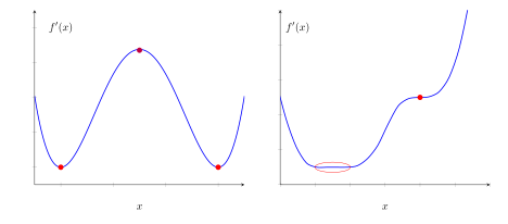
Figure 4.2: Two graphs illustrating the types of convergence for a stochastic gradient (SG) algorithm. In the left graph, an SG algorithm for minimization would converge to one of the two local minima or the local maximum indicated by the filled (red) circles, where which one it reaches depends on the starting point and the noise. In the right graph, the SG algorithm could converge to the saddle point indicated by the filled (red) circle or would eventually bounce between points in the circled (in red) interval unless the noise goes to zero. As long as the gradient estimate remains appropriately noisy, the SA algorithm would eventually move away from the local maximum in the left graph and away from the saddle point in the right graph.
If the set \(H\) specified in Theorem 4.2 consists of a single point, then the convergence would be to that point. Otherwise, the meaning of convergence to a set is depicted by two graphs in Figure 4.2. If all the elements in the set are disconnected, then convergence would be to a single point in the set, with the specific point to which the algorithm converges depending on the initial condition, the step size sequence, and the noise, as illustrated in the left graph of Figure 4.2, which contains two local minima and one local maximum. If some of the points are connected, then the algorithm could “bounce” between such points and not converge to a single point, as illustrated in the right graph of Figure 4.2, which contains a flat local minimal region and a saddle point. “Unstable” points such as local maxima (in minimization problems) and saddle points can be avoided by ensuring that the gradient estimate is suitably noisy, to be described in more detail below.
Since the ODE tracked by the iteration (4.4) is \(\dot{\theta} = -\nabla f(\theta)\), we know that its stationary points will be local maxima or minima, saddle points, or points of inflection. If these points are isolated, then the algorithm (4.4) will a.s. converge to a (possibly) sample path-dependent stationary point. Under additional assumptions, one can ensure convergence to a local minimum, thereby avoiding convergence to local maxima or saddle points. One such assumption is that the stationary points are hyperbolic, i.e., the Hessian \(\nabla^2 f\) does not have eigenvalues on the imaginary axis. Then locally, it has a ‘stable manifold’ of dimension equal to the number of eigenvalues in the left half plane and an unstable manifold with the complementary dimension. A trajectory on the former converges to the stationary point along the stable manifold, whereas one on the latter moves away from it on the unstable manifold. A trajectory initiated anywhere else also eventually moves away. Thus, if there is at least one unstable eigenvalue, the trajectories move away from the stationary point except on the stable manifold, a set of zero Lebesgue measure. Hence, if the noise is omnidirectional, i.e., rich in all directions in a certain precise sense, the iterations will be pushed away from the stable manifold often enough for the iterates to move away from the stationary point for good, a.s. Then the iterates will a.s. converge to a local minimum, where there are no unstable directions. In case the conditions on noise cannot be verified for the problem at hand, one can possibly add extraneous i.i.d. zero mean noise and have an SA update iteration of the form
\[ \begin{align*} \theta_{n+1} = \theta_n - a(n) (\widehat\nabla f(\theta_n) + \varphi_{n}), \tag{4.6} \end{align*} \]
where \(\varphi_{n}\) is extraneous noise added to ensure that the algorithm avoids saddle points/local maxima. A simple choice is to sample \(\varphi_n\) from the \(d\)-dimensional unit sphere uniformly. In practice, it may not be necessary to add such a noise factor extraneously, since the algorithm has an inherent noise component in the gradient estimates. We discuss escaping saddle points in more detail in Chapter 7.
4.1.2 Stochastic gradient algorithm using unbiased (direct) gradient estimates
We begin by considering the case when unbiased direct (noisy) gradient measurements are available. This would correspond to the setting of infinitesimal perturbation analysis (IPA) based estimators where information on direct sample performance gradients is available and one does not resort to zeroth-order gradient estimation methods.
To solve (1.1), a stochastic gradient algorithm would update as follows:
\[ \begin{align*} \theta_{n+1} = \theta_n - a(n) \widehat\nabla f(\theta_n), \tag{4.7} \end{align*} \]
where \(\widehat\nabla f(\theta_n)\) is an estimate of the gradient \({\nabla} f(\theta_n)\), and \(\{a(n)\}\) are (pre-determined) step-sizes satisfying standard Robbins-Monro step-size conditions (see A4.3 below).
In a zeroth-order setting, the gradient information is not directly available, and instead, the optimization algorithm has oracle access to noise-corrupted function measurements. We also present in the latter case, an analysis of the resulting stochastic approximation scheme with gradient estimates obtained from zeroth-order information. Such estimates are not unbiased, but feature a parameter that can reduce the bias at the cost of variance. As mentioned, before getting to zeroth-order gradient estimation, we shall cover a simpler setting where unbiased gradient information is indeed available, i.e., \(\E( \widehat\nabla f(\theta_n) ) = \nabla f(\theta_n)\). In this case, the algorithm in (4.7) becomes an instance of the seminal stochastic approximation scheme proposed by Robbins and Monro in 1951. The latter algorithm was proposed to find the zeroes of a function, and in the case of (4.7), the function of interest is \(\nabla f\).
The algorithm in (4.7) can be shown to converge to local optima of \(f\), and we make this claim precise, by starting with the necessary assumptions below.
Assumption A4.1.
\(\nabla f\) is a Lipschitz continuous \(\R^d\)-valued function.
Assumption A4.2.
\(\widehat\nabla f(\theta_n)\) is an unbiased estimate of the gradient \({\nabla} f(\theta_n)\), i.e., \(\E\left[ \widehat\nabla f(\theta_n) \mid \F_n \right] = \nabla f(\theta_n)\), where \(\F_n = \sigma(\theta_m,m \le n)\) denotes the underlying sigma-field. Further, there exists \(\sigma >0\) such that
\[ \begin{align*} \EE{ \l\widehat\nabla f(\theta_n) - \EE{\left.\widehat\nabla f(\theta_n)\right| \F_n}\r^2 } \le \sigma^2 < \infty. \tag{4.8} \end{align*} \]
Assumption A4.3.
The step-sizes satisfy \(\sum_n a(n)=\infty \text{ and } \sum_n a(n)^2 < \infty.\)
Assumption A4.4.
The iterates \(\{\theta_n,n\ge 0\}\) are stable, i.e., \(\sup_n \left\| \theta_n \right\| < \infty\), a.s.
Before presenting a proof of this result, we discuss below the assumptions made. First, the continuity requirement on the objective function \(h(\theta)\) in A4.1 is standard to the analysis of stochastic approximation algorithms. Indeed for the setting considered here, \(h(\theta)=-\nabla f(\theta)\). Second, the unbiasedness condition in A4.2 is not satisfied in a zeroth-order optimization setting, where the gradient information is directly unavailable, and instead, one needs to infer this through measurements of the objective function at any query point. In the following section, we shall discuss the simultaneous perturbation trick, leading to asymptotically-unbiased gradient estimates, in place of A4.2.
Third, the condition on step-sizes in A4.3 are standard requirements in stochastic approximation, and the reader is referred to the next chapter for a brief motivation (or Chapter 2 of (Borkar 2022) for a detailed description). Fourth, the stability requirement in A4.4 is standard in the analysis of stochastic approximation algorithms, and this assumption was discussed in detail in the previous chapter, see Section 2.3.
Proof of Theorem 4.4
For proving Theorem 4.4, we shall invoke Theorem 4.2.
Proof.
The update in (4.7) is equivalent to
\[ \begin{align*} \theta_{n+1} = \theta_n - a(n)\bigg(\nabla f(\theta_n) + \eta_n \bigg), \tag{4.9} \end{align*} \]
where \(\eta_n = \widehat\nabla f(\theta_n) - \E\left[\left.\widehat\nabla f(\theta_n) \right| \F_n\right]\) is a martingale difference term. The equivalent update rule above used the fact that \(\E\left[\left.\widehat\nabla f(\theta_n) \right| \F_n\right]= \nabla f(\theta_n)\), which holds by assumption A4.2.
The mean ODE underlying (4.1) is
\[ \begin{align*} \dot{\theta} = -\nabla f(\theta), \tag{4.10} \end{align*} \]
with limit set \(H=\big\{\theta:\nabla f(\theta)\big)=0\big\}\).
To apply Theorem 4.2, we verify a few conditions below.
Since \(\beta_n = 0, \ \forall n\), A2.2 is trivially satisfied.
To verify A2.4, we first recall a martingale inequality attributed to Doob (also given as (2.1.7) on pp. 27 of (Kushner and Clark 1978)):
\[ \begin{align*} \Prob{ \sup_{m\geq 0} \left\|W_m\right\| \geq \epsilon} \le \dfrac{1}{\epsilon^2} \lim_{m\rightarrow \infty} \E \left\|W_m\right\|^2. \tag{4.11} \end{align*} \]
Applying the inequality above to \(W_m\triangleq \sum_{i=n}^{m} a(i) \eta_i\), \(m\ge n\) and \(n\ge 1\), we obtain
\[ \begin{align*} &P\left( \sup_{m\geq n} \left\|\sum_{i=n}^{m} a(i) \eta_i\right\| \geq \epsilon \right) \le \dfrac{1}{\epsilon^2} \E \left\| \sum_{i=n}^{\infty} a(i) \eta_i\right\|^2 = \dfrac{1}{\epsilon^2} \sum_{i=n}^{\infty} a(i)^2 \E\left\| \eta_i\right\|^2. \tag{4.12} \end{align*} \]
The last equality above follows by observing that, for \(k < l\), \(\E\left[\eta_k\tr \eta_l\right] = \E\left[\eta_k\tr \E\left[\left.\eta_l\right|\F_k\right]\right]=0\).
Now, using the square-summability of the stepsize in A4.3 and (4.8) in A4.2, we have
\[ \begin{align*} P\left( \sup_{m\geq n} \left\|\sum_{i=n}^{m} a(i) \eta_i\right\| \geq \epsilon \right) \le \dfrac{1}{\epsilon^2} \sum_{i=n}^{\infty} a(i)^2 \E\left\| \eta_i\right\|^2\le \dfrac{\sigma^2}{\epsilon^2} \lim_{n\rightarrow\infty} \sum_{i=n}^{\infty} a(i)^2 \\ \rightarrow 0 \textrm{ as } n\rightarrow \infty. \end{align*} \]
Thus, \(\{\theta_n\}\) converges a.s. to the set \(\bar H\) by an application of Theorem 4.2.
\(\square\)
4.1.3 Stochastic gradient algorithm using (zeroth-order) biased gradient estimates
We now consider the case where we have zeroth-order gradient estimates constructed from (noisy) function measurements obtained from an oracle. The bias in these gradient estimates is seen to vanish asymptotically as we allow the sensitivity parameter \(\delta\) to tend to zero.
We analyze the following stochastic gradient algorithm:
\[ \begin{align*} \theta_{n+1} = \theta_n - a(n) \widehat\nabla f(\theta_n), \tag{4.13} \end{align*} \]
where \(\widehat\nabla f(\theta_n)\) is formed using the unified estimate from the previous chapter, which is recalled below.
\[ \begin{align*} \widehat\nabla f(\theta_n) = \left(\frac{ y_n^+ - y_n^-}{2\delta_n}\right) V(n), \tag{4.14} \end{align*} \]
where \(y_n^+= f(\theta_n+\delta_n U(n))+\xi_n^+\), and \(y_n^- = f(\theta_n- \delta_n U(n))+\xi_n^-\). The reader is referred to Chapter 3 for a variety of choices for the random vectors \(U(n),V(n)\).
For the analysis of this algorithm, we require the following assumptions in addition to A4.4 listed earlier: Let \(\F_n=\sigma(\theta_i, i\le n, U(i), V(i), i<n, \xi_i^\pm, i<n)\), \(n\geq 1\) denote a sequence of sigma fields.
Assumption A4.5.
The noise factors \(\xi^\pm\) in (4.14) satisfy
\[ \begin{align*} \E[\xi_n^+-\xi_n^- |\, \F_n] &= 0, \text{~~ and ~~} \E [ (\xi_n^{+} - \xi_n^-)^{2} |\, \F_n] \le \sigma^2 <\infty\,, \,\forall n\ge 1. \tag{4.15} \end{align*} \]
Assumption A4.6.
The objective function \(f:\R^d\rightarrow \R\) satisfies
\[ \begin{align*} \E [ f(\theta_n \pm \delta_n U(n))^{2} \mid \F_n] \le B <\infty, \forall n. \tag{4.16} \end{align*} \]
Assumption A4.7.
The step-sizes \(a(n)\) and perturbation constants \(\delta_n\) are positive, for all \(n\) and satisfy
\[ a(n), \delta_n \rightarrow 0\text{ as } n \rightarrow \infty, \sum_n a(n)=\infty \text{ and } \sum_n \left(\frac{a(n)}{\delta_n}\right)^2 <\infty. \]
Assuming \(f\in\C^3\), and using Assumptions A4.5–A4.6, it is possible to infer the following bias and variance bounds on the gradient estimator (4.14):
\[ \begin{aligned}\forall n\ge 1, \norm{ \EE{\widehat\nabla f(\theta_n)\mid \F_n} \!-\! \nabla f(\theta_n) } \le C_1\delta_n^2, \textrm { and } \\ \EE{\norm{ \widehat\nabla f(\theta_n) - \EE{\left.\widehat\nabla f(\theta_n)\right| \F_n} }^2} \le \frac{C_2}{\delta_n^2}, \end{aligned} \tag{4.17} \]
for some constants \(C_1\) and \(C_2\). A straightforward adaptation of the proof of Proposition 3.1 leads to the bound in (4.17).
The result below establishes asymptotic convergence of (4.13) to stationary points of \(f\) and the bounds in (4.17) is a crucial ingredient in the proof.
Theorem 4.5.
Assume A4.5–A4.7, A4.4, and that \(f\) is \(L\)-smooth as well as three times continuously differentiable with bounded third derivative, i.e., \(f\in \C^3\). Let \(\bar{H}\) denote the largest invariant set contained in \(\{ \theta \mid \nabla f(\theta) = 0 \}\). Then, the iterates \(\theta_n\), \(n\geq 1\), updated according to (4.13), satisfy
\[ \theta_n \rightarrow \bar H \text{ a.s. as } n\rightarrow \infty. \]
Proof.
We first rewrite the update rule (4.13) as follows:
\[ \begin{align*} \theta_{n+1} = \theta_n - a(n)(\nabla f(\theta_n) + \eta_n + \beta_n), \tag{4.18} \end{align*} \]
where \(\eta_n = \widehat \nabla f(\theta_n) - \E\left[\widehat \nabla f(\theta_n) \mid \F_n\right]\) is a martingale difference term, and \(\beta_n = \E\left[\widehat \nabla f(\theta_n) \mid \F_n\right] - \nabla f(\theta_n)\) is the bias in the gradient estimate.
Convergence of (4.13) can be inferred from Theorem 4.2, provided we verify the necessary assumptions, and we do this verification below.
\(f\) is \(L\)-smooth implies A2.1.
From (4.17), we have \(\beta_n = O(\delta_n^2)\). In conjunction with A4.7, we have \(\beta_n \rightarrow 0\), verifying A2.2.
Applying Doob’s martingale inequality, \(W_m = \sum_{i=n}^{m} a(i) \eta_i\), \(m\ge n\) and \(n\ge 1\), we obtain
\[ \begin{align*} \mathbb P\left( \sup_{m\geq n} \left\|\sum_{i=n}^{m} a(i) \eta_i\right\| \geq \epsilon \right) &\le \dfrac{1}{\epsilon^2} \E \left\| \sum_{i=n}^{\infty} a(i) \eta_i\right\|^2 \\ &= \dfrac{1}{\epsilon^2} \sum_{i=n}^{\infty} a(i)^2 \E\left\| \eta_i\right\|^2, \tag{4.19} \end{align*} \]
where, as in the proof of Theorem 4.4, the last equality used \(\E\left[\eta_k\tr \eta_l\right] =0\) for \(k < l\). This verifies A2.4.
Using (4.17), we have
\[ \begin{align*} &\E\left\| \eta_n\right\|^2 \le \frac{C_2}{\delta_n^2}. \tag{4.20} \end{align*} \]
Now, substituting the bound in (4.20) into (4.19), we obtain
\[ \begin{align*} \lim_{n\rightarrow\infty} P\left( \sup_{m\geq n} \left\| \sum_{i=n}^{m} a(i) \eta_i\right\| \geq \epsilon \right) \le \dfrac{C_2}{\epsilon^2} \lim_{n\rightarrow\infty} \sum_{i=n}^{\infty} \frac{a(i)^2}{\delta_i^2} =0. \end{align*} \]
The equality above follows from A4.7, as a consequence of
\(\sum_n \left(\frac{a(n)}{\delta_n}\right)^2 <\infty\).
The main claim now follows by an application of Theorem 4.2.
\(\square\)
Remark 4.1.
The above result shows that the ODE tracked by (4.13) is (4.5). Except for one gradient estimation scheme, all the other schemes that we consider (see Chapter 3) track the ODE (4.5). However, for the case when the truncated Cauchy smoothed functional (TCSF) gradient estimator (3.31) is used, it can be seen that the ODE tracked is the following:
\[ \dot{\theta}(t) = -c_2\nabla f(\theta), \tag{4.21} \]
with \(c_2>0\). While the asymptotic convergence in this case is also to the stable fixed points of the ODE that is qualitatively the same as (4.5), the effect of the multiplicative constant \(c_2>0\) manifests in the speed of convergence of the ODE’s trajectories to the ODE’s stable fixed points. In particular, \(c_2>1\) would result in faster convergence of the trajectories of (4.21) as compared to that of the ODE (4.5). As mentioned, the latter ODE is the one tracked by all the other algorithms studied so far.
4.2 Asymptotic convergence: A differential inclusions approach
We now consider the case when gradient estimators such as (4.14) are considered but where \(\delta>0\) is held constant. This ensures that there is a bias in the gradient estimates that however does not asymptotically vanish as with the previous case.
4.2.1 Assumptions
We make the following assumptions:
Assumption A4.8.
\(f: \mathbb{R}^d\rightarrow \mathbb{R}\) is continuously differentiable. Furthermore,
\(\norm{\nabla f(\theta)} \leq \tilde{K}(1+\norm{\theta})\) for all \(\theta\in \mathbb{R}^d\), for some \(\tilde{K}>0\).
Assumption A4.9.
\(\{\eta_n\}\) is a square-integrable martingale difference sequence w.r.t. the filtration \(\{\F_n\}\), where \(\F_n = \sigma(\theta_m, m\leq n, \eta_m, m<n), n\geq 0\). Further,
\[ \E[\norm{\eta_n}^2 \mid \F_n] \leq K_1(1+\norm{\theta_n}^2), \]
for some constant \(K_1>0\).
Assumption A4.10.
\(a(n)> 0\), \(\forall n\). Further, \(\sum_n a(n)=\infty\) and \(\sum_n a(n)^2 <\infty.\)
Assumption A4.11.
\(\sup_n \left\| \theta_n \right\| < \infty\) w.p. \(1\).
A sufficient condition for the second part of Assumption A4.8 (in addition to \(f\) being continuously differentiable) is that the function \(\nabla f\) is a Lipschitz continuous function of \(\theta\). This is because in such a case
\[ \norm{\nabla f(\theta_1) - \nabla f(\theta_2)} \leq Q \norm{\theta_1-\theta_2}, \]
for some constant \(Q>0\) and for any \(\theta_1,\theta_2\in \mathbb{R}^d\). Then by letting \(\theta_1=\theta\) and \(\theta_2 =0\), we get
\[ \norm{\nabla f(\theta)} - \norm{\nabla f(0)} \le \norm{\nabla f(\theta)- \nabla f(0)} \leq Q\norm{\theta}, \]
implying \(\norm{\nabla f(\theta)} \leq \tilde{K}(1+\norm{\theta})\) with \(\tilde{K} = \max(Q, \norm{\nabla f(0)})\).
Assumption A4.9 is on the noise sequence \(\{\eta_n\}\). From the manner in which it is defined, viz., \(\eta_n = \widehat\nabla f(\theta_n) - \E\left[\widehat\nabla f(\theta_n) \mid \F_n\right]\) and the various forms of the gradient estimators \(\widehat\nabla f(\theta_n)\) discussed previously and the assumptions on the measurement noise there, it can be easily seen that this condition will be satisfied.
Assumption A4.10 is on the step size sequence and is a standard requirement in stochastic approximation schemes. The condition on non-summability of the step size is needed to track the asymptotic behaviour of the limiting differential equation or inclusion as the case may be. The second condition ensures, in particular, that the errors due to noise asymptotically vanish.
Finally, assumption A4.11 is necessary to establish convergence of gradient-descent scheme but is a non-trivial requirement. Certain sufficient conditions for stability of stochastic approximation schemes that rely mainly on the underlying ODE and a certain scaling limit of the same are given in (Borkar and Meyn 1999). For the case of stochastic recursive inclusions (SRI), i.e., stochastic approximations with set-valued maps, similar conditions have recently been provided in (A. Ramaswamy and Bhatnagar 2016, 2018). In particular, (A. Ramaswamy and Bhatnagar 2018) considers a gradient recursion with errors in the setting of SRI and provides sufficient conditions for stability of the scheme. We present these conditions from (A. Ramaswamy and Bhatnagar 2018) in the subsection following the convergence proof. Prior work, for instance, (Benaïm 1996; Kushner and Clark 1978; Kushner and Yin 2003) show convergence of stochastic approximation assuming stability of the stochastic iterates. Further, (Benaïm, Hofbauer, and Sorin 2005) proves the almost sure convergence of SRI again assuming stability of the iterates. As mentioned earlier, if one is unable to ensure stability of the stochastic iterates, a common approach is to project these to a large enough compact set that would ensure boundedness of the iterates. This however comes at the cost of introducing spurious fixed points on the projection set boundary to which the recursion might converge as well, see (Kushner and Clark 1978; Kushner and Yin 2003) for detailed analyses of projected stochastic approximations.
4.2.2 Proof of Convergence
Let \(G(\theta) = \nabla f(\theta) + \overline{B}_\epsilon(0)\), where \(\overline{B}_\epsilon(0)\) is a closed ball of radius \(\epsilon>0\) around the origin. In other words, \(G(\theta)=\overline{B}_\epsilon(\nabla f(\theta))\) is a closed ball of radius \(\epsilon>0\) around \(\nabla f(\theta)\).
Lemma 4.6.
The set-valued map \(G\) is a Peano map.
Proof.
Recall Definition A.6 for definition of Peano map. We shall verify the three conditions (i)-(iii) of Definition A.6. As noted earlier, for any \(\theta \in \R^d\), \(G(\theta)\) is a closed ball in \(\mathbb{R}^d\) of radius \(\epsilon\) centred at \(\nabla f(\theta)\). Thus, it is clearly convex and compact. Now for any \(y\in G(\theta)\),
\[ \begin{align*} \norm{y} &\leq \norm{\nabla f(\theta)} + \norm{y-\nabla f(\theta)} \\ &\leq \tilde{K}(1+\norm{\theta}) +\epsilon \\ &\leq \bar{K}(1+\norm{\theta}), \end{align*} \]
where \(\bar{K} = \tilde{K}+\epsilon\). The second inequality above follows from the smoothness assumption A4.8. Since \(y\) above is arbitrary, it follows that
\[ \sup_{y\in G(\theta)} \norm{y} \leq \bar{K}(1+\norm{\theta}). \]
Thus \(G(\theta)\) is pointwise bounded.
Finally, consider a sequence \(\theta_n, n\geq 0\) of parameters and another sequence \(y_n, n\geq 0\) of points such that \(y_n \in G(\theta_n)\), \(\forall n\). Further, let \(\theta_n \rightarrow \theta\) and \(y_n \rightarrow y\) as \(n\rightarrow \infty\). Now given \(\delta>0\) small, let \(N\) be large enough so that \(\norm{y_n-y} < \delta/2\) and similarly \(\norm{\nabla f(\theta_n) - \nabla f(\theta)} < \delta/2\), respectively, \(\forall n>N\). Then,
\[ \begin{align*} \norm{y-\nabla f(\theta)} & \leq & \norm{y-y_n} + \norm{y_n - \nabla f(\theta_n)} \\ & & + \norm{\nabla f(\theta_n) - \nabla f(\theta)} \\ &\leq \epsilon + \delta. \end{align*} \]
Since \(\delta>0\) is arbitrary, let \(\delta \rightarrow 0\). It then follows that \(\norm{y-\nabla f(\theta)} \leq \epsilon\), implying that \(y\in G(\theta)\). Thus \(G\) is also upper-semicontinuous and the claim follows.
\(\square\)
Consider now the Differential Inclusion (DI):
\[ \dot{\theta}(t) \in -G(\theta(t)). \tag{4.22} \]
Here \(-G(\theta(t))\) is used to denote the set \(\{-g \mid g \in G(\theta(t))\}\). The next result follows directly from (Benaïm, Hofbauer, and Sorin 2005).
Proof.
The claim follows from Theorem 3.6 and Lemma 3.8 of (Benaïm, Hofbauer, and Sorin 2005).
\(\square\)
Consider also the associated ODE that would result from the case of \(\epsilon=0\):
\[ \begin{align*} \dot{\theta}_t = -\nabla f(\theta_t). \tag{4.23} \end{align*} \]
This will be the case when either the information on the gradient \(\nabla f(\theta)\) is fully known for all \(\theta\) and a (true) gradient scheme with noise is used or else the sensitivity parameter \(\delta\) is replaced by a slowly decreasing \(\delta_n \rightarrow 0\). Both of these cases have been analysed for their convergence in Section 4.1.
As seen in Section 4.1, in the second case above, the square summability requirement of the step size sequence \(\{a(n)\}\) is considerably tightened. More specifically, the condition \({\displaystyle \sum_n a(n)^2 <\infty}\) in A4.10 is replaced by the more stringent requirement \({\displaystyle \sum_n \left(\frac{a(n)}{\delta_n}\right)^2 <\infty}\) in A4.7. The latter has the effect of significantly constraining the learning rates in the update recursion.
Let \(\mathcal{M}\) denote the minimum set of \(f\) and suppose the regular values of \(f\), i.e., \(\theta\) for which \(\nabla f(\theta) \not= 0\) are dense in \(\mathbb{R}^d\), then the chain recurrent set of \(f\) is a subset of it’s minimum set, see Proposition 4 of Hurley (Hurley 1995). As shown earlier, the gradient descent scheme without errors (i.e., with \(\epsilon=0\)), will converge to \(\mathcal{M}\) almost surely.
We now state Theorem 3.1 of (Benaïm, Hofbauer, and Sorin 2012) adapted to the setting considered here..
Theorem 4.8.
Given \(\delta > 0\), \(\exists \epsilon(\delta) > 0\) such that the chain recurrent set of (4.22) is within the \(\delta\)-open neighborhood of the chain recurrent set of (4.23) for all \(\epsilon \leq \epsilon(\delta)\).
It follows as a consequence of Theorem 4.7 and Theorem 4.8 that (4.2) with \(\epsilon < \epsilon(\delta)\) (cf. Theorem 4.8) converges almost surely to \(N^{\delta}(\mathcal{M})\).
4.2.3 A Set of Stability Conditions for Stochastic Recursive Inclusions
We now present a set of conditions from (A. Ramaswamy and Bhatnagar 2016, 2018) that ensure that the stochastic recursive inclusion (4.2) remains stable, i.e., that \(\sup_n \norm{\theta_n} <\infty\) a.s., that was the last assumption for our analysis of the recursion (4.2). The conditions that we present are a generalization of stability conditions for stochastic approximation presented in (Borkar and Meyn 1999).
Recall from Lemma 4.6 that \(G\) is a Peano or Marchaud map. For each integer \(c \ge 1\), let
\[ G_c (\theta) := \left\{ \frac{y}{c} \mid y \in G(c\theta) \right\}. \]
Let
\[ G_\infty (\theta) := \overline{co}(\mbox{Limsup}_{c \to \infty} G_c (\theta)), \]
where
\[ \mbox{Limsup}_{x_n\rightarrow x} J(x_n) = \{y\in\mathbb{R}^d\mid \liminf_{x_n\rightarrow x}d(y,J(x_n))=0\}, \]
see Definition A.7. Given \(A \subseteq \mathbb{R}^d\), the convex closure of \(A\), denoted by \(\overline{co}(A)\), is the closure of the convex hull of \(A\). It is worth noting that \(Limsup_{c \to \infty} G_c (\theta)\) is non-empty for every \(\theta \in \mathbb{R}^d\). It is also shown in Lemma 1 of (A. Ramaswamy and Bhatnagar 2018) that \(G_\infty\) is Marchaud. Thus, from (Aubin and Cellina 1984), the DI \(\dot{\theta}(t) \in -G_\infty (\theta(t))\) has at least one solution that is absolutely continuous.
We make the following additional assumptions:
Assumption A4.12.
\(\dot{\theta}(t) \in -G_\infty (x (t))\) has an attractor set \(\mathcal{A}\) such that \(\mathcal{A} \subseteq B_a (0)\) for some \(a > 0\) and \(\overline{B}_a (0)\) is a fundamental neighborhood of \(\mathcal{A}\).
Since \(\mathcal{A} \subseteq B_a (0)\) is compact, we have that \(\underset{\theta \in \mathcal{A}}{\sup} \lVert \theta \rVert < a\).
Assumption A4.13.
Let \(c_{n} \ge 1\) be an increasing sequence of integers such that \(c_{n} \uparrow \infty\) as \(n \to \infty\). Further, let \(\theta_n \ \rightarrow \ \theta\) and \(y_{n} \ \rightarrow \ y\) as \(n \ \rightarrow \infty\), such that \(y_{n} \in G_{c_{n}}(\theta_n)\), \(\forall n\), then \(y \in G_{\infty}(\theta)\).
It can be shown that the existence of a global Lyapunov function for \(\dot{\theta}(t) \in -G_\infty (\theta(t))\) is sufficient to guarantee that A4.12 holds. Further, A4.13 is satisfied when \(\nabla f\) is Lipschitz continuous.
A detailed proof of this result is given in Theorem 1 of (A. Ramaswamy and Bhatnagar 2018). What is important to note here as also with the original result of (Borkar and Meyn 1999) (that was for the case of stochastic updates involving single-valued functions as opposed to set-valued maps as considered above), both the additional assumptions A4.12 and A4.13 involve only deterministic systems, more precisely scaled Differential Inclusions. Asymptotic stability properties of these systems and in particular the limiting system are enough to guarantee stability of the original stochastic recursions.
If there is no estimation error and no noise, then it is straightforward to see that \(\theta_n\) converges a.s. to \(K\). We now argue that a similar conclusion holds even in the presence of gradient estimation error and noise elements in function measurements. The relevant technical result that is necessary to claim convergence of \(\theta_n\) is Kushner-Clark lemma. To apply the latter lemma we verify a few conditions:
“\(\beta_n \rightarrow 0\) almost surely” \(\leftarrow\) holds since we assume \(\delta_n \rightarrow 0\) and \(\beta_n = O(\delta_n^2)\)
“\(\forall \epsilon>0\), \(\lim_{n\rightarrow\infty} \underbrace{P\left( \sup_{m\geq n} \left\| \sum_{i=n}^{m} a(i) \delta_i\right\| \geq \epsilon \right)}_{(*)} = 0.\)”
\[ \begin{align*} &(*) \le \dfrac{1}{\epsilon^2} \E \left\| \sum_{i=n}^{\infty} a(i) \delta_i\right\|^2 = \dfrac{1}{\epsilon^2} \sum_{i=n}^{\infty} a(i)^2 \E\left\| \delta_i\right\|^2\le \dfrac{C}{\epsilon^2} \lim_{n\rightarrow\infty} \sum_{i=n}^{\infty} \frac{a(i)^2}{\delta_i^2} \rightarrow 0 \end{align*} \]
\(K\) is an asymptotically stable attractor for the ODE: holds since \(f\) itself serves as a Lyapunov function.
Thus, \(\theta_n\) converges a.s. to the set \(K\).
4.3 Bibliographic remarks
The steps involved in establishing the convergence analysis of stochastic approximation algorithms with gradient estimators mirrors largely similar analysis for broader stochastic approximation algorithms dealt with in Chapter 2, see (Benaïm 1996; Borkar 2022). Convergence analyses of zeroth-order stochastic gradient algorithms with diminishing step-sizes are for instance, available in (Spall 1992, 1997) for the case of two and one-sided SPSA, in (Prashanth et al. 2017) for the case of RDSA, as well as (Prashanth et al. 2020) for deterministic perturbation RDSA.
Stochastic recursive inclusions or stochastic approximation with set-valued maps have been analysed for the first time in (Benaïm, Hofbauer, and Sorin 2005). The recursion there involves a set-valued map with a martingale difference noise sequence and assumes stability of the stochastic iterates. The works in (A. Ramaswamy and Bhatnagar 2016, 2021) provide the first and only available sets of stability conditions for such recursions. Stability conditions for stochastic recursive inclusions with non-ergodic Markov noise are available in (A. Ramaswamy and Bhatnagar 2019).
The works in (Arunselvan Ramaswamy and Bhatnagar 2016; Yaji and Bhatnagar 2020) present the first convergence analyses of two-timescale stochastic recursive inclusions with set-valued maps on both timescales. In (Yaji and Bhatnagar 2018), the analysis of stochastic recursive inclusions with set-valued maps and Markov noise in addition, has been conducted for the first time and in (Yaji and Bhatnagar 2018), the same in the two-timescale case is conducted in (Yaji and Bhatnagar 2020). The Markov noise is assumed to be dependent on the parameter sequence and in addition, depends on an additional control-valued sequence, and furthermore is assumed to have multiple stationary distributions. This combination makes it the hardest so far case of stochastic inclusions that has been analysed in the literature. Such algorithms are however seen to have applications in stochastic optimization as well as reinforcement learning. For instance, an application of (Karmakar and Bhatnagar 2018) on two-timescale stochastic approximation with Markov noise was studied on an application of off-policy gradient temporal difference learning algorithms (Sutton et al. 2009). Finally, the material on convergence of a zeroth-order stochastic gradient algorithm for a fixed \(\delta\)-parameter is based on (A. Ramaswamy and Bhatnagar 2018), where a corresponding set-valued map is obtained and analysed.