5 Non-asymptotic analysis of stochastic gradient algorithms
We consider a SG algorithm for solving (1.1), with an update iteration of the form:
\[ \begin{align*} \theta_{n+1} = \theta_n - a(n) \widehat \nabla f(\theta_n), n\ge 0. \tag{5.1} \end{align*} \]
We analyze the algorithm above with inputs from either an unbiased gradient oracle or a biased one, i.e., corresponding to the cases where \(\EE{ \widehat\nabla f(\theta)\mid \theta}=\nabla f(\theta)\) and \(\EE{ \widehat\nabla f(\theta)\mid \theta}=\nabla f(\theta) + O(\delta^2)\), with \(\delta\) denoting the perturbation constant (see Chapter 3), respectively. The analysis in the former case serves as a useful contrast to the biased case, since the proof technique is similar, while there is a loss in convergence rate when one moves from an unbiased to a biased gradient oracle.
We consider an SG algorithm that runs for \(N\) iterations, and outputs a (possibly random) point \(\theta_R\), that could be chosen based on the iterates \(\theta_1,\ldots, \theta_{N}\). For a general SG algorithm, we consider different performance metrics based on the nature of the underlying objective. More precisely, we consider the following cases:
(i) convex; (ii) strongly convex; and (ii) non-convex.
In case (i), we provide bounds on the optimization error, i.e.,
\(\E\left(f(\theta_R) - f(\theta^*) \right)\), where \(\theta^*\) is a minimum of \(f\), whereas in case (ii), we establish bounds on the parameter error \(\E \l \theta_R - \theta^*\r^2\). On the other hand, in case (iii), i.e., when the objective is non-convex, it is difficult to bound the optimization/parameter errors. A popular alternative is to establish local convergence. i.e., to a point where the gradient of the objective is small (cf. (Ghadimi and Lan 2013; Bottou, Curtis, and Nocedal 2018)). The following definition makes the optimization objectives apparent in all the cases studied in this chapter.
Definition 5.1.
Let \(\theta_R \in \R^d\) be the output of a SG algorithm and \(\epsilon > 0\) be a target accuracy, then:
If \(f\) is non-convex, \(\theta_R\) is called an \(\epsilon\)-stationary point of (1.1), if \(\E \left\| \nabla f \left(\theta_{R}\right)\right\|^{2} \le \epsilon\);
If \(f\) is convex, \(\theta_R\) is called an \(\epsilon\)-optimal point of (1.1), if
\(\E [f \left(\theta_{R}\right)] - f(\theta^*) \le \epsilon\), where \(\theta^*\) is a minimizer of \(f\).If \(f\) is strongly convex, \(\theta_R\) is called an \(\epsilon\)-optimal point of (1.1), if \(\E\left[\l\theta_{R} - \theta^*\r^2\right] \le \epsilon\), where \(\theta^*\) is the unique minimizer of \(f\).
The SG algorithms are judged using the iteration complexity, which is defined below.
Definition 5.2.
For a given \(\epsilon>0\), the iteration complexity of an algorithm \(\mathcal A\) is the number of iterations of \(\mathcal A\) before finding an \(\epsilon\)-stationary (resp. \(\epsilon\)-optimal) point for a non-convex (resp. convex/strongly-convex) objective function.
For a gradient descent type algorithm, results from deterministic optimization lead to complexity bounds listed in Table 5.1, cf. (Wright and Recht 2022, chap. 3).
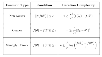
Table 5.1: Summary of iteration complexities of a gradient descent algorithm for deterministic smooth optimization. Here iteration complexity is the number of iterations \(n\) required to satisfy the condition specified in the second column. Here \(\theta^*\) denotes an optimum of \(f\), \(\theta_0\) is the starting point of the gradient descent algorithm, \(\mu\) is the strong-convexity parameter, and \(L\) is the smoothness constant.
The bounds in Table 5.1 are useful to compare against the corresponding cases in the stochastic case that we consider in this chapter. Moreover, as we shall see later, the case of biased gradient oracle results in bounds that are weaker than the unbiased counterpart.
For the bounds in this chapter, we consider a variant of SG algorithm, namely randomized stochastic gradient (RSG), which was proposed in (Ghadimi and Lan 2013). This is a well-known scheme that provides a non-asymptotic bound on a random iterate visited by a SG algorithm. More precisely, suppose \(\theta_1,\ldots,\theta_m\) be the iterates visited along a sample path of a SG algorithm that is run for \(m\) iterations. Then, the RSG algorithm would return an iterate \(\theta_R\) that is picked randomly from the set \(\{\theta_1,\ldots,\theta_m\}\). For the case where \(\theta_R\) is picked uniformly at random from the set mentioned above, the RSG scheme for picking the aforementioned random iterate resembles the well-known Polyak-Ruppert iterate averaging scheme (Polyak and Juditsky 1992; Ruppert 1985) for stochastic approximation. The latter scheme performs averaging of all the iterates \(\{\theta_i,\ i=1,\ldots,m\}\), while RSG achieves the same effect, except that the averaging happens in expectation. Algorithm 2 presents the pseudocode of RSG algorithm that takes as input the probability mass function \(P_R(\cdot)\) for picking a random variable from the set \(\{1,\ldots,m\}\). The bounds we present are for the special case where \(P_R\) is the discrete uniform distribution over the aforementioned set.
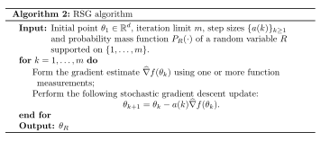
In this chapter, we provide non-asymptotic bounds for Algorithm 2 with unbiased and biased gradient information, respectively, for three different assumptions on the underlying objective, namely convex, strongly convex and non-convex. In a zeroth-order setting, the RSG algorithm is provided gradient estimates formed using the simultaneous perturbation method described in Chapter 3.
The rest of this chapter is organized as follows: Sections 5.1–5.3 present the non-asymptotic bounds with proofs for non-convex, convex, and strongly convex functions, respectively. In Section 5.4, we present two settings where the non-asymptotic bounds for the RSG algorithm features improved dimension dependence, as compared to those in Sections 5.1–5.3. In Section 5.5, we discuss a zeroth-order model variant, where the function measurements are biased. In Section 5.6, we present a minimax lower bound for an algorithm that has access to gradient estimates that satisfy a bias-variance tradeoff (e.g., see (4.3)). In Section 5.7, we outline the connection between smooth optimization in a zeroth-order setting and bandit convex optimization.
5.1 The non-convex case
We begin by considering the case of a non-convex objective function \(f:\mathbb{R}^d\rightarrow\mathbb{R}\).
5.1.1 RSG with an unbiased gradient oracle
As a gentle start, first, we provide bounds for the simple “unbiased gradient” model, and subsequently analyze the other challenging model involving biased gradients.
In this model, we assume access to a stochastic first-order oracle, which for a given \(\theta_k\) outputs a random estimate \(\widehat\nabla f(\theta_k)\) of the gradient of \(f\). We assume that the gradient estimate \(\widehat\nabla f(\theta_k)\) satisfies the following assumption:
Assumption A5.1.
Let \(\F_k=\sigma(\theta_i, i\le k)\). Recall \(\E_k\) denotes the expectation w.r.t. \(\F_k\). For any \(k \ge1\), we have
\(\E_k \left[ \widehat\nabla f(\theta_k)\right] = \nabla f \left(\theta_k\right) ,\)
\({ \E_k \left[ \left\| \widehat\nabla f(\theta_k) - \nabla f \left(\theta_k\right)\right\|^{2}\right] \leq \sigma^{2} },\) for some parameter \(\sigma \ge 0\).
From the above, it is apparent that \(\widehat\nabla f(\theta_k)\) is an unbiased estimate of \(\nabla f(\theta_k)\) with bounded variance.
The results provide a bound on the gradient norm after \(m\) iterations of RSG. As mentioned earlier, under a non-convex objective, bounding the optimization error, i.e., \(f(\theta_R) - f(\theta^*)\) is difficult, where \(\theta^*\) is a local optima. However, a popular alternative is to show that the RSG algorithm converges to a point, where the gradient of the objective is small (quantified by a bound on the squared norm of the gradient) (cf. (Ghadimi and Lan 2013; Bottou, Curtis, and Nocedal 2018)).
Theorem 5.1.
(Unbiased gradients: Non-convex case) Suppose \(f\) is \(L\)-smooth and satisfies A5.1. Suppose that the RSG algorithm is run with the stepsize sequence set as
\[ \begin{align*} a(k) = a, \forall k \textrm{ with } a=\min \bigg\{\frac{1}{L}, \frac{c}{\sqrt{m}}\bigg\}, \tag{5.2} \end{align*} \]
for some constant \(c > 0\). Then, for any \(m \ge 1\), we have
\[ \begin{align*} & \E \left[ \left\| \nabla f \left(\theta_{R}\right)\right\|^{2}\right] \le \frac{ 2 L D_f}{{ m }} + \frac{1}{\sqrt{m}} \bigg[ \frac{ 2 D_f}{{ c }} + L \sigma^2 {c} \bigg], \end{align*} \]
where \(R\) is uniformly distributed over \(\{1,\dots,m \}\), \(\theta^*\) is an optimal solution to (1.1), and
\[ \begin{align*} D_f = f(\theta_1) - f(\theta^*). \tag{5.3} \end{align*} \]
Proof.
Since \(f\) is \(L\)-smooth, we have
\[ \begin{align*} f \left(\theta_{k+1}\right) & \leq f \left(\theta_k\right) + \left\langle \nabla f \left(\theta_k\right) , \theta_{k+1} - \theta_k\right\rangle + \frac { L } {2} \left\| \theta_{k+1} - \theta_k\right\|^{2} \\ & = f \left(\theta_k\right) - a(k) \left\langle \nabla f \left(\theta_k\right) , \widehat\nabla f(\theta_k)\right\rangle + \frac { L } {2} a(k)^{2} \left\| \widehat\nabla f(\theta_k)\right\|^{2} \end{align*} \]
Using \(\E_k \left[ \widehat\nabla f(\theta_k)\right] = \nabla f \left(\theta_k\right) ,\) and the following inequality1:
\[ \E_k \left[ \left\| \widehat\nabla f(\theta_k)\right\|^{2}\right] \le \left\| \E_k \left[ \widehat\nabla f(\theta_k)\right] \right\| ^{2} + \sigma^2, \]
we obtain
\[ \begin{align*} &\E_k [f \left(\theta_{k+1}\right) ] \\ & \leq f \left(\theta_k\right) - a(k) \left\| \nabla f \left(\theta_k\right)\right\|^{2} + \frac { L } {2} a(k)^{2} \left[ \left\| \nabla f \left(\theta_k\right)\right\|^{2} +\sigma^2\right] \\ & = f \left(\theta_k\right) - \left( a(k) - \frac { L } {2} a(k)^{2}\right) \left\| \nabla f \left(\theta_k\right)\right\|^{2} + \frac { L } {2} a(k)^{2} \sigma^{2}. \tag{5.4} \end{align*} \]
Re-arranging the terms above and setting \(a(k) = a, \forall k \geq 1\), we obtain
\[ \begin{align*} & a \left\| \nabla f \left(\theta_k\right)\right\|^{2} \leq \frac{2 \left[ f \left(\theta_k\right) - \E_k [f \left(\theta_{k+1}\right)]\right]}{\left( 2- La\right)} + \frac{L a^{2} \sigma^{2}}{\left( 2- La\right)} \end{align*} \]
Now, summing up the above inequality for \(k=1\) to \(m\), we obtain
\[ \begin{align*} &a \sum_{k=1}^{ m } \left\| \nabla f \left(\theta_k\right)\right\|^{2} \leq 2 \sum_{k=1}^{ m } \frac{ \left[ f \left(\theta_k\right) - \E_k [f \left(\theta_{k+1}\right)]\right]}{\left( 2- La\right)} + \frac{ m L \sigma^2 a^{2} }{\left( 2- La\right)}. \end{align*} \]
Taking total expectations on both sides of above equation, and using \(\E \left[ f \left(\theta_k\right)\right] \ge f(\theta^*)\), for all \(k\ge 1\), we obtain
\[ \begin{align*} & a\sum_{k=1}^{ m } \E \left\| \nabla f \left(\theta_k\right)\right\|^{2} \le \frac { 2 \left(f(\theta_1) - f(\theta^*)\right)} { \left( 2- La\right)} + \frac{ m L \sigma^2 a^2}{\left( 2- La\right)}. \end{align*} \]
Since \(\theta_R\) is picked uniformly at random from \(\{\theta_1,\ldots,\theta_m\}\) and \(a\le 1/L\), we have
\[ \begin{align*} \E \left[ \left\| \nabla f \left(\theta_{R}\right)\right\|^{2}\right]&= \frac{1}{m}\sum_{k=1}^{ m} \E \left\| \nabla f \left(\theta_k\right)\right\|^{2} \\ & \le \frac{1}{{ m }a } \left[ \frac { 2 D_f} { \left( 2- La \right)} + L \sigma^2 { m }\frac{ a^2}{\left( 2- La \right)}\right] \\ & \le \frac{1}{{ m }a } \left[ { 2 D_f} + L \sigma^2 { m }{ a^2}\right] \\ & = \frac{ 2 D_f}{{ m }a} + L \sigma^2 a \\ & \le \frac{ 2 D_f}{{ m }} max\bigg\{L, \frac{\sqrt{m}}{c}\bigg\} + L \sigma^2 \frac{c}{\sqrt{m}} \\ & \le \frac{ 2 L D_f}{{ m }} + \frac{ 2 D_f}{{ c \sqrt{m} }} + L \sigma^2 \frac{c}{\sqrt{m}} \\ & = \frac{ 2 L D_f}{{ m }} + \frac{1}{\sqrt{m}}\left[ \frac{ 2 D_f}{{ c }} + L \sigma^2 {c}\right]. \end{align*} \]
The claim follows.
\(\square\)
5.1.2 RSG with a biased gradient oracle
We make the following assumptions for the non-asymptotic analysis of RSG algorithm in the zeroth-order setting:
Assumption A5.2.
There exists a constant \(B > 0\) such that \(\| \nabla f ( x ) \|_1 \leq B, \forall x \in \R^d\).
Assumption A5.3.
The gradient estimate \(\widehat \nabla f(\theta_k)\) satisfies the following inequalities for all \(k\ge 1\):
\[ \begin{align*} \l\mathbb { E }_{k} \left[ \widehat \nabla f(\theta_k) \right] - \nabla f \left( \theta_ { k } \right)\r & \leq c_1 \delta^2, \tag{5.5} \end{align*} \]
and
\[ \begin{align*} &\mathbb { E }_{k} \left[ \left\| \widehat \nabla f(\theta_k) \right\|^{2} \right]\le \left\| \mathbb { E }_{k} \left[ \widehat \nabla f(\theta_k) \right] \right\| ^{2} + \frac{c_2 }{ \delta^2}. \tag{5.6} \end{align*} \]
In the above, \(\mathbb { E }_{k}\) is shorthand for \(\mathbb { E }(\cdot \mid \F_k)\), with \(\F_k\) denoting the sigma-field \(\sigma\left(\theta_i, i\le k\right)\).
As mentioned before, in the non-convex case, the gradient norm is a standard benchmark for quantifying the convergence rate of stochastic gradient algorithms. The main result concerning RSG’s non-asymptotic performance is presented below.
Theorem 5.2.
Suppose the objective function \(f\) is \(L\)-smooth (see Definition 3.1), and assumptions A5.2–A5.3 hold. Suppose that the RSG algorithm is run with the stepsize \(a(k)=a\) and perturbation constant \(\delta(k)=\delta\) for each \(k=1,\ldots,m\), where
\[ \begin{align*} a = min \bigg\{\frac{1}{L}, \frac{1}{m^{2/3}}\bigg\}, \text{ } \delta = \frac{1}{m^{1/6}}, \text{ } \forall k \geq 1. \tag{5.7} \end{align*} \]
Then, choosing \(\theta_R\) uniformly at random from \(\{\theta_1,\ldots,\theta_m\}\), we have
\[ \begin{align*} & \mathbb { E } \left\| \nabla f \left( \theta_{ R } \right) \right\| ^ { 2 } \le \frac{ 2 L (f(\theta_1) - f(\theta^*)) }{{ m }} + \frac{\mathcal{K}_1}{m^{1/3}}, \tag{5.8} \end{align*} \]
where \(\mathcal{K}_1 = { 2D_f d^{4/3}} + \frac{4 B c_1}{d^{5/3}}+ \frac{L c_1^2 }{ d^{11/3}m} + {L c_2 d^{1/3}}\), constants \(c_1, c_2\) are defined in A5.3, \(B\) is as defined in A5.2,
\[ \begin{align*} D_f = f(\theta_1) - f(\theta^*), \tag{5.9} \end{align*} \]
and \(\theta^*\) is a global optima of \(f\).
Remark 5.1.
From the bound in the result above, it is easy to see that an order \(\mathcal{ O} \left(\frac{1}{\epsilon^3}\right)\) iterations of the RSG algorithm are enough to find a point \(\theta_R\) that satisfies \(\E\left\| \nabla f \left( \theta_{ R } \right) \right\| ^ { 2 } \le \epsilon\).
Remark 5.2.
In comparison to the unbiased gradient information case handled in the previous section, the \(\mathcal{ O} \left(\frac{1}{m^{1/3}}\right)\) bound obtained here is weaker. This drop in rate is owing to the bias-variance tradeoff in the gradient estimates, i.e., choosing a very small perturbation constant \(\delta\) improve the accuracy of the gradient estimate at the cost of increased variance, see Assumption A5.3. However, with additional structure, the rate can be improved to \(\mathcal{ O} \left(\frac{1}{m^{1/2}}\right)\). We mention two such settings next. First, in the case of common random noise, discussed earlier in Subsection 3.3.4, we have \(f(\theta)=\E_\xi(F(\theta,\xi))\). Assuming \(F\) is smooth in \(\theta\), for any given \(\xi\), it is possible to establish a \(\mathcal{ O} \left(\sqrt{\frac{d}{m}}\right)\) bound on the gradient norm square, i.e., \(\E\left\| \nabla f \left( \theta_{ R } \right) \right\| ^ { 2 }\). Notice that this bound improves both the dependency on dimension \(d\) as well number of iterations \(m\). The proof for such a result is analogous to the proof of Theorem 5.2 given below, and we leave it as an exercise. The second setting with improved bounds is that of sparse optimization. Assuming the gradient is \(s\)-sparse, i.e., \(\norm{\nabla f(x)}_0\le s, \forall x\), it is possible to establish a \(\mathcal{ O} \left(\sqrt{\frac{\log d}{m}}\right)\) bound on the gradient norm square. In comparison to the first setting with smooth sample performance, this bound has a better dependence on the dimension, and this is due to the sparsity assumption.
Proof.
(Theorem 5.2)
Since \(f\) is \(L\)-smooth, we have
\[ \begin{align*} f \left( \theta_ { k + 1 } \right) & \leq f \left( \theta_ { k } \right) + \left\langle \nabla f \left( \theta_ { k } \right) , \theta_ { k + 1 } - \theta_ { k } \right\rangle + \frac { L } { 2 } \left\| \theta_ { k + 1 } - \theta_ { k } \right\| ^ { 2 } \\ & \leq f \left( \theta_ { k } \right) - a \left\langle \nabla f \left( \theta_ { k } \right) , \widehat \nabla f(\theta_k) \right\rangle + \frac { L } { 2 } a ^ { 2 } \left\| \widehat \nabla f(\theta_k) \right\| ^ { 2 } . \tag{5.10} \end{align*} \]
Taking expectations with respect to the sigma field \(\F_{k}\) on both sides of (5.10), and using (5.5) and (5.6) from A5.3, we obtain
\[ \begin{align*} & \E_{k} \left[f \left( \theta_ { k + 1 } \right)\right] \\ & \leq \E_{k} \left[f \left( \theta_ { k } \right) \right] - a \left\langle \nabla f \left( \theta_ { k } \right) , \nabla f \left( \theta_ { k } \right) + c_1 \delta^2 \mathbf{1}_{d \times 1} \right\rangle \\ & \quad + \frac { L } { 2 } a ^ { 2 } \left[ \left\| \mathbb { E }_{k} \left[ \widehat \nabla f(\theta_k) \right] \right\| ^{2} + \frac{c_2}{ \delta^2} \right] \\ & \leq f \left( \theta_ { k } \right) - a \left\| \nabla f \left( \theta_ { k } \right) \right\| ^ { 2 } + c_1 \delta^2 a \E_{k} \| \nabla f \left( \theta_ { k } \right) \|_1 \\ & \quad + \frac { L } { 2 } a ^ { 2 } \left[ \left\| \nabla f \left( \theta_ { k } \right) \right\| ^ { 2 } + 2 c_1 \delta^2 \E_{k} \| \nabla f \left( \theta_ { k } \right) \|_1 + {d}c_1^2 \delta^4 + \frac{c_2}{ \delta^2} \right] \tag{5.11} \\ & \leq f \left( \theta_ { k } \right) - \left( a - \frac { L } { 2 } a ^ { 2 } \right) \left\| \nabla f \left( \theta_ { k } \right) \right\| ^ { 2 } + c_1 \delta^2 B \left( a + L a ^ { 2 } \right) \tag{5.12} \\ &\qquad+ \frac { L } { 2 } a ^ { 2 } \left[ d c_1^2 \delta^4 + \frac{c_2}{ \delta^2}\right], \end{align*} \]
where we have used the fact that \(- \|y\|_1 \leq \sum_{i=1}^{N} y_i\) for any vector \(N\)-vector \(y\), in arriving at the inequality (5.11). The last inequality follows from the fact that \(\| \nabla f \left( \theta_ { k } \right) \|_1 \leq B\) by assumption A5.2. Re-arranging the terms, we obtain
\[ \begin{align*} &a \left\| \nabla f \left( \theta_ { k } \right) \right\| ^ { 2 } \leq \frac{2}{\left( 2 - { L } a \right) } \bigg[ f \left( \theta_ { k } \right) - \E_{k} f \left( \theta_ { k + 1 } \right) \bigg. \\ & \quad \bigg. + c_1 \delta^2 \left( a + L a ^ { 2 } \right)B \bigg] + \frac{{ L } a ^ { 2 }}{\left( 2 - { L } a \right) } \left[ dc_1^2 \delta^4 + \frac{c_2}{ \delta^2}\right]. \end{align*} \]
Now, summing up the inequality above for \(k = 1\) to \(m\), and taking expectations, we obtain
\[ \begin{align*} & \sum _ { k = 1 } ^ { m} a \E_{m} \left\| \nabla f \left( \theta_ { k } \right) \right\| ^ { 2 } \\ & \leq 2 \sum _ { k = 1 } ^ { m} \frac{ \left(\E_{m} f \left( \theta_ { k } \right) - \E_{m} f \left( \theta_{k+1} \right) \right)}{\left( 2 - { L } a \right) } + 2 m c_1 \delta^2 B \left( \frac{ a + L a ^ { 2 } }{ 2 - { L } a }\right) \\ & \quad + L m \frac{ a ^ { 2 }}{\left( 2 - { L } a \right) } \left[ dc_1^2 \delta^4 + \frac{c_2}{ \delta^2}\right] \\ & = 2 \left[\frac { f \left( \theta_ { 1 } \right) } { \left( 2- { L } a \right) } - \frac { \mathbb { E }_{m} \left[ f \left( \theta_ { m + 1 } \right) \right] } { \left( 2- { L } a(m) \right) } \right] \\ & \quad + 2 m c_1 \delta^2 B \left( \frac{ a + L a ^ { 2 } }{ 2 - { L } a }\right) + L m \frac{ a ^ { 2 }}{\left( 2 - { L } a \right) } \left[ dc_1^2 \delta^4 + \frac{c_2}{ \delta^2}\right]. \end{align*} \]
Using \(\mathbb { E }_{m} \left[ f \left( \theta_ { k } \right) \right] \ge f(\theta^*)\), we obtain
\[ \begin{align*} \sum _ { k = 1 } ^ { m } a \E_{m} \left\| \nabla f \left( \theta_ { k } \right) \right\| ^ { 2 } &\leq \frac { 2 \left(f(\theta_1) - f(\theta^*) \right)} { \left( 2- { L } a \right)} + 2 m c_1 \delta^2 B \left( \frac{ a + L a ^ { 2 } }{ 2 - { L } a }\right) \\ & \quad + L m \frac{ a ^ { 2 }}{\left( 2 - { L } a \right) } \left[ dc_1^2 \delta^4 + \frac{c_2}{ \delta^2}\right]. \end{align*} \]
Using the fact that \(\theta_R\) is picked uniformly at random from \(\{\theta_1,\ldots,\theta_m\}\), we obtain
\[ \begin{align*} \mathbb { E } \left[ \left\| \nabla f \left( \theta_{ R } \right) \right\| ^ { 2 } \right] &\le \frac{1 }{m a} \left[\frac { 2 D_f} { \left( 2- { L } a \right)} + 2 B m c_1 \delta^2 \left( \frac{ a + L a ^ { 2 } }{ 2 - { L } a }\right) \right. \\ &\quad\qquad \left. + L m \frac{ a ^ { 2 }}{\left( 2 - { L } a \right) } \left[ dc_1^2 \delta^4 + \frac{c_2}{ \delta^2}\right] \right]. \tag{5.13} \end{align*} \]
Next, we simplify the bound obtained above by substituting the step-size and perturbation constant values specified in (5.7) as follows:
\[ \begin{align*} & \mathbb { E } \left[ \left\| \nabla f \left( \theta_ { R } \right) \right\| ^ { 2 } \right] \\ & \le \frac{1}{{ m }a } \left[ { 2 D_f} + 4m a B c_1\delta^2 + { L m a ^ { 2 }}\left[ d c_1^2\delta^4 + \frac{c_2}{\delta^2}\right] \right] \tag{5.14} \\ & \le \frac{ 2 D_f}{{ m }} max\bigg\{L, {m^{2/3}}\bigg\} + 4 B \left(\frac{c_1 }{m^{1/3}} \right)+ { L }\left[ \frac{dc_1^2}{m^{2/3}} + \frac{c_2}{m^{-1/3}}\right] \frac{1}{m^{2/3}} . \tag{5.15} \end{align*} \]
In the above, the inequality (5.14) follows by using the fact that \(a \leq 1/L\), while the inequality (5.15) uses the choice of \(\delta\) in (5.7). The main claim follows follows by rearranging terms in (5.15).
\(\square\)
5.2 The convex case
We now study the non-asymptotic performance of the RSG algorithm presented earlier, assuming that the objective is convex and smooth. The main result that provides a non-asymptotic bound for RSG algorithm with gradient estimates satisfying A5.3 is given below.
Theorem 5.3.
Suppose the objective function \(f\) is \(L\)-smooth (see Definition 3.1), and convex. Assume A5.3 holds. Suppose that the RSG algorithm is run for \(m\) iterations with stepsize \(a\), perturbation constant \(\delta\) set as defined in (5.7). Let \(\theta_R\) be chosen uniformly at random from \(\{\theta_1,\ldots,\theta_m\}\). Then, for any \(m \ge 1\), we have
\[ \begin{align*} & \E \left[ f \left( \theta_ { R } \right) \right] - f (\theta^{*}) \le \frac{ L D^2}{{ m }} + \frac{\mathcal{K}_1}{m^{1/3}}, \end{align*} \]
where \(\mathcal{K}_1 = D^2 + 4 \sqrt{d} D c_1 \delta^2 + \frac{ d c_1^2 \delta^4 }{m } + c_2\), constants \(c_1\) and \(c_2\) are specified in A5.3, and
\[ \begin{align*} D = \| \theta_1 - \theta^*\|, \tag{5.16} \end{align*} \]
with \(\theta^*\) denoting a global optima of \(f\).
The case of unbiased gradient information leads to a \(O(1/\sqrt{m})\) bound and the proof is a complete parallel argument to the one employed for the biased case in the result above, and we omit the details.
Remark 5.3.
From the result above, it is apparent that an \(\mathcal{ O} \left(\frac{1}{\epsilon^3}\right)\) number of iterations is necessary to find a point that satisfies \(\E \left[ f \left( \theta_ { R } \right) \right] - f (\theta^{*})\le \epsilon\). Moreover, this rate is not improvable in a minimax sense for a gradient-based algorithm with inputs from a biased gradient oracle, which we formalize in the next section.
Remark 5.4.
For the special case of noise originating from a common random number sequence that was discussed earlier in Subsection 3.3.4, it is possible to obtain an improved bound of the order \(\mathcal{ O} \left(\sqrt{\frac{d}{m}}\right)\). This improvement comes from the fact that the gradient estimate variance does not blow up as the perturbation constant \(\delta\) goes to zero, see Proposition 3.5. The proof of this improved bound follows arguments similar to those employed in the proof of Theorem 5.3. We omit the details.
Remark 5.5.
The bound in Theorem 5.3 above is for a random iterate \(\theta_R\). Using a different step size choice that decays in a geometric fashion, and a radically different proof technique, it is possible to infer a bound of the same order, i.e., \(O\left(m^{-1/3}\right)\) for the last iterate \(\theta_m\). The reader is referred to Section IV-B of (Bhavsar and Prashanth 2022) for the details. Note that the last iterate is preferred over a random iterate in practice, and hence, it is desirable to obtain bounds for the last iterate. For the non-convex case, to the best of our knowledge, there are no bounds available for a stochastic gradient algorithm with inputs from a biased gradient oracle.
Proof.
(Theorem 5.3)
Let \(\Delta_k = \widehat\nabla f(\theta_k) - \nabla f(\theta_k)\) and \(\omega _ { k } = \left\| \theta_ { k } - \theta^* \right\|, \forall k \geq 1\). Then for any \(k = 1,\dots,m\), we have
\[ \begin{align*} \omega _ { k + 1 } ^ { 2 } & = \| \theta_{k+1} - \theta^* \|^2 \\ & = \|\theta_{k} - a \widehat\nabla f(\theta_k) - \theta^* \|^2 \\ & = \omega _ { k } ^ { 2 } - 2 a \left\langle \widehat\nabla f(\theta_k) , \theta_ { k } - \theta^* \right\rangle + a ^ { 2 } \left\| \widehat\nabla f(\theta_k) \right\| ^ { 2 }. \tag{5.17} \end{align*} \]
Taking expectations with respect to the sigma field \(\F_{k}\) on both sides of (5.17), and using (5.5), (5.6), we obtain
\[ \begin{align*} \mathbb { E }[\omega _ { k + 1 } ^ { 2 }] & \leq \E [\omega _ { k } ^ { 2 }] - 2 a \left\langle \nabla f(\theta_k) , \theta_ { k } - \theta^* \right\rangle - 2 a \E \left[\left\langle\Delta_k , \theta_ { k } - \theta^* \right\rangle\right] \\ & \text{ } + a ^ { 2 } \bigg[ \left\| \E_k \left[ \widehat\nabla f(\theta_k)\right] \right\| ^{2} + \frac{c_2}{ \delta^2} \bigg] \\ & \leq \E [\omega _ { k } ^ { 2 }] - 2 a \left\langle \nabla f \left( \theta_ { k } \right) , \theta_ { k } - \theta^* \right\rangle + 2 a c_1 \delta^2\| \theta_ { k } - \theta^* \|_1 \\ & \text{ } + a ^ { 2 } \bigg[ \| \nabla f \left( \theta_ { k } \right) \| ^ { 2 } + 2 \sqrt{d} c_1 \delta^2 \| \nabla f \left( \theta_ { k } \right) \| + dc_1^2\delta^4 + \frac{c_2}{ \delta^2} \bigg], \tag{5.18} \end{align*} \]
where the last inequality follows from the fact that \(- \sum_{i=1}^{N} \theta_i \leq \|X\|_1\) for any vector \(X\). Now, using the fact that \(f\) is convex, we have
\[ \left\| \nabla f \left( \theta_ { k } \right) \right\| ^ { 2 } \leq L \left\langle \nabla f \left( \theta_ { k } \right) , \theta_ { k } - \theta^* \right\rangle. \]
Further, since \(f\) is \(L\)-smooth, \(\| \nabla f(\theta_k) \| \leq L \| \theta_k - \theta^* \|\). Plugging these inequalities in (5.18), we obtain
\[ \begin{align*} \mathbb { E } [\omega _ { k + 1 } ^ { 2 }] & \leq \E [\omega _ { k } ^ { 2 }] - 2 a \left\langle \nabla f \left( \theta_ { k } \right) , \theta_ { k } - \theta^* \right\rangle + 2 a c_1 \delta^2\| \theta_ { k } - \theta^* \|_1 \\ & \quad + a ^ { 2 } \bigg[ L \left\langle \nabla f \left( \theta_ { k } \right) , \theta_ { k } - \theta^* \right\rangle + 2\sqrt{d} c_1 \delta^2 L \| \theta_k - \theta^* \| \\ & \qquad\qquad + dc_1^2\delta^4+ \frac{c_2}{ \delta^2} \bigg] \\ & \leq \E [\omega _ { k } ^ { 2 }] - (2a _ { k } - L a^2)\left[ f \left( \theta_ { k } \right) - f (\theta^* ) \right] \\ & \quad + 2 \sqrt{d} \omega_k c_1 \delta^2 a + L a^2) + a ^ { 2 } \bigg[ dc_1^2\delta^4+ \frac{c_2}{ \delta^2} \bigg], \end{align*} \]
where the last inequality follows from the fact that \(f(\cdot)\) is convex along with \(\| X \|_1 \leq \sqrt{d} \| X \|\) for any vector \(X\). Re-arranging the terms, we obtain
\[ \begin{align*} & a \left[ f \left( \theta_ { k } \right) - f (\theta^*) \right] \\ &\leq \frac{1}{(2 - L a)} \bigg[ \omega _ { k } ^ { 2 } - \mathbb { E } [\omega _ { k +1 } ^ { 2 }] + 2 \sqrt{d} \omega c_1 \delta^2 (a + L a^2) + a ^ { 2 } \bigg(d c_1^2\delta^4+ \frac{c_2}{ \delta^2} \bigg) \bigg]. \end{align*} \]
Now summing up the inequality above from \(k = 1\) to \(m\) and taking expectations, we obtain
\[ \begin{align*} \sum _ { k = 1 } ^ { m } a \E_m\left[ f \left( \theta_ { k } \right) - f (\theta^{*}) \right] & \leq \sum _ { k = 1 } ^ { m } \frac{\E_m [\omega _ { k } ^ { 2 }] - \E_m[\omega _ { k + 1 } ^ { 2 }]}{(2 - L a)} \\ & + 2 \sqrt{d} \sum _ { k = 1 } ^ { m } \E_m \left[ \omega _ { k } \right] c_1 \delta^2 \frac{ a + L a^2) }{(2 - L a)} \\ & + \sum _ { k = 1 } ^ { m } \frac{a^2 }{(2-L a)}\bigg( d c_1^2\delta^4 + \frac{c_2}{ \delta^2}\bigg) \\ & = \frac { \omega _ { 1 } ^ { 2 } } { \left( 2- { L } a \right) } - \frac { \E_m \left[ \omega _ { m+1 } ^ { 2 } \right] } { \left( 2- { L } a \right) } \\ & \quad + 2 \sqrt{d} \sum _ { k = 1 } ^ { m } \E_m \left[ \omega _ { k } \right] c_1 \delta^2 \frac{(a + L a^2) }{(2 - L a)} \\ & \quad + \sum _ { k = 1 } ^ { m } \frac{a ^ { 2 } }{(2- L a)}\bigg(d c_1^2\delta^4 + \frac{c_2}{ \delta^2}\bigg) \\ & \leq \frac { D^2} { \left( 2- { L } a \right)} + 2 \sqrt{d }D \sum _ { k = 1 } ^ { m } c_1 \delta^2 \frac{ (a + L a^2) }{(2 - L a)} \\ & \quad + \sum _ { k = 1 } ^ { m } \frac{a ^ { 2 } }{(2-L a)}\bigg( d c_1^2\delta^4 + \frac{c_2}{ \delta^2}\bigg) \end{align*} \]
where the last inequality follows by using (5.16), i.e., \(\E_m \left[ \omega _ { k } \right] \leq D\). Combining the above result with the fact that \(\theta_R\) is picked uniformly at random from \(\{\theta_1,\ldots,\theta_m\}\), we obtain
\[ \begin{align*} & \mathbb { E } \left[ f \left( \theta_ { R } \right) \right] - f (\theta^{*}) \\ &\le \frac{1}{m a } \bigg[ \frac { D^2} { \left( 2- { L } a \right)} + 2\sqrt{d} D \sum _ { k = 1 } ^ { m } c_1 \delta^2 \frac{ (a + L a^2) }{(2 - L a)} \\ & \qquad + \sum _ { k = 1 } ^ { m } \frac{a ^ { 2 } }{(2-L a)}\bigg( d c_1^2\delta^4 + \frac{c_2}{ \delta^2}\bigg) \bigg], \tag{5.19} \end{align*} \]
Using (5.7) in (5.19), we obtain
\[ \begin{align*} &\mathbb { E } \left[ f \left( \theta_R \right) \right] - f (\theta^{*}) \\ & \le \frac{1}{ m a } \bigg[ \frac { D^2} { \left( 2- { L } a \right)} + 2 \sqrt{d} D \sum _ { k = 1 } ^ { m } c_1 \delta^2 \frac{ a + L a^2) }{(2 - L a)} \\ & \qquad + \sum _ { k = 1 } ^ { m } \frac{a ^ { 2 } }{(2- L a)}\bigg(d c_1^2\delta^4 + \frac{c_2}{ \delta^2}\bigg) \bigg] \\ & \le \frac{1}{{ m }a } \left[ { D^2} + 4 \sqrt{d} D m a c_1\delta^2 + m a^2\bigg(d c_1^2\delta^4 + \frac{c_2}{\delta^2}\bigg) \right], \tag{5.20} \end{align*} \]
where the final inequality follows by using the fact that \(a \leq 1/L\). The main claim follows by using the definition of \(a, \delta\) given in (5.7) followed by simple algebraic manipulations.
\(\square\)
5.3 The strongly-convex case
In this section, we present non-asymptotic analysis for the SG algorithm (5.1) under a strongly convex objective, which is made precise in the definition below.
Definition 5.3.
A continuously differentiable function \(f\) is \(\mu\)-strongly convex if the following condition holds for any \(\theta,\theta'\):
\[ \begin{align*} f(\theta') \geq f(\theta) + \nabla f(\theta)^T (\theta'-\theta) + \frac{\mu}{2}\norm{\theta'-\theta}^2. \end{align*} \]
For a brief introduction to strong-convexity, the reader is referred to Appendix D. As in the previous sections, we consider unbiased as well as biased gradient information. We begin with the unbiased gradient case in the next section.
5.3.1 SG with unbiased gradient information
We consider the following update iteration:
\[ \begin{align*} \theta_{k+1} = \theta_k - a(k) \widehat \nabla f(\theta_k). \tag{5.21} \end{align*} \]
We first state and prove a result for the case of a constant step size.
Theorem 5.4.
Let \(f\) be a \(\mu\)-strongly convex function. Assume A5.1. Then, the SG algorithm governed by (5.21) and with \(a(k) = a\) s.t. \(0 < a L < 1\), satisfies
\[ \begin{align*} \E[f(\theta_{m}) - f(\theta^*)] \leq&\ \frac{a L\sigma^2}{2\mu} + \left(1 - a \mu\right)^{m-1} \left(f(\theta_1) - f(\theta^*) - \frac{ a L\sigma^2}{2\mu}\right). \tag{5.22} \end{align*} \]
Proof.
From the initial passage in the proof of Theorem 5.1, we have
\[ \begin{align*} \E_k[f(\theta_{k+1})] - f(\theta_k) \leq - a(k)(1 - \frac{1}{2}a(k) L ) \|\nabla f(\theta_k)\|_2^2 + \frac{1}{2} a(k)^2 L \sigma^2. \end{align*} \]
Since \(a(k) = a\) and \(0 < a L < 1\), we have
\[ \begin{align*} \E_k[f(\theta_{k+1})] - f(\theta_k) \leq - \frac{1}{2}a \|\nabla f(\theta_k)\|_2^2 + \frac{1}{2} a^2 L \sigma^2. \tag{5.23} \end{align*} \]
Since \(f\) is \(\mu\)-strongly convex, the following inequality, which is well-known as the Polyak-Lojasiewicz (PL) condition holds2:
\[ f(\theta)-f(\theta^*) \le \frac{1}{2\mu}\|\nabla f(\theta)\|_2^2,\ \forall \theta. \]
Using the above inequality in (5.23), we obtain
\[ \begin{align*} \E_k[f(\theta_{k+1})] - f(\theta_k) \leq - \mu a \left(f(\theta_k)-f(\theta^*)\right) + \frac{1}{2} a^2 L \sigma^2. \tag{5.24} \end{align*} \]
Subtracting \(f(\theta^*)\) on both sides and re-arranging, we obtain
\[ \begin{align*} \E_k[f(\theta_{k+1}) - f(\theta^*)] \leq (1 - a \mu)[f(\theta_k) - f(\theta^*)] + \frac{1}{2}a^2L\sigma^2. \tag{5.25} \end{align*} \]
Taking expectations followed by straightforward simplifications, we obtain
\[ \begin{align*} & \E[f(\theta_{k+1}) - f(\theta^*)] - \frac{a L\sigma^2}{2\mu} \\ &\leq (1 - a \mu) \E[f(\theta_k) - f(\theta^*)] + \frac{a^2 L\sigma^2}{2} - \frac{a L\sigma^2}{2\mu} \\ &= (1 - a \mu) \left(\E[f(\theta_k) - f(\theta^*)] - \frac{a L\sigma^2}{2\mu}\right). \tag{5.26} \end{align*} \]
Using \(a < 1/L\) by assumption, and \(\mu \le L\), we have3
\[ a \mu < \frac{\mu}{L} \le 1. \]
A repeated application of the above inequality leads to the following bound:
\[ \begin{align*} \E[f(\theta_{m}) - f(\theta^*)] \leq&\ \frac{a L\sigma^2}{2\mu} + \left(1 - a \mu\right)^{m-1} \left(f(\theta_1) - f(\theta^*) - \frac{ a L\sigma^2}{2\mu}\right). \tag{5.27} \end{align*} \]
The claim follows.
\(\square\)
Remark 5.6.
Using the bound on the optimization error (or the difference in function values) in the result above, we can establish a bound on the parameter error as follows: From \(\mu\)-strong convexity of \(f\), we have
\[ f(\theta) + \nabla f(\theta)\tr(\tilde\theta-\theta) + \frac{\mu}{2}\norm{\tilde\theta-\theta}^2 \le f(\tilde\theta). \]
At \(\theta=\theta^*\), \(\nabla f(\theta^*)=0\), implying
\[ \norm{\tilde\theta-\theta}^2 \le \frac{2}{\mu}\left(f(\tilde\theta)-f(\theta^*)\right). \]
Thus, a bound on the difference in function values implies a bound on the parameter error.
Remark 5.7.
Taking limits as \(n\rightarrow\infty\), the bound in (5.22) converges to \(\frac{a L\sigma^2}{2\mu}\). This observation implies that a constant step size stochastic gradient algorithm does not converge to the optima, and instead gets to within a ball around the optima.
Next, we consider the case of a diminishing step size.
Theorem 5.5.
Let \(f\) be a \(\mu\)-strongly convex function. Assume A5.1. Then, the SG algorithm governed by (5.21) and with \(a(k) = \frac{c}{k+1}\) s.t. \(\frac{1}{\mu} < c \le L\), satisfies
\[ \begin{align*} \E\left[f(\theta_{m}) - f(\theta^*)\right] \leq&\ \frac{1}{m+1} \max\left\{ \frac{c^2 L\sigma^2}{2(c\mu -1)},2\left(f(\theta_1) - f(\theta^*)\right) \right\}. \tag{5.28} \end{align*} \]
Proof.
We prove by induction. The base case holds trivially. Assuming the claim holds for \(m\), we show that it holds for \(m+1\).
From (5.4), we have
\[ \begin{align*} \E_k[f(\theta_{k+1})] - f(\theta_k)] & \leq - a(k)(1 - \frac{1}{2}a(k) L ) \|\nabla f(\theta_k)\|_2^2 + \frac{1}{2} a(k)^2 L \sigma^2 \\ & \le - a(k)\|\nabla f(\theta_k)\|_2^2 + \frac{1}{2} a(k)^2 L \sigma^2 \tag{Since $a(k) L \le 1$} \\ & \le - a(k) \mu\left(f(\theta_k) - f(\theta^*)\right) + \frac{1}{2} a(k)^2 L \sigma^2 \tag{PL-condition} \end{align*} \]
Thus,
\[ \begin{align*} \E[f(\theta_{k+1})] - f(\theta^*)] & \le (1- a(k) \mu)\E[f(\theta_k) - f(\theta^*)] + \frac{1}{2} a(k)^2 L \sigma^2. \end{align*} \]
Using the induction hypothesis, the form of the step size \(a(k)\) and letting \(K=\max\left\{ \frac{c^2 L\sigma^2}{2(c\mu-1)},2\left(f(\theta_1) - f(\theta^*)\right) \right\}\), we obtain
\[ \begin{align*} \E[f(\theta_{m+1})] - f(\theta^*)] & \le \left(1- \frac{c\mu}{m+1}\right)\frac{K}{m+1} + \frac{c^2 L \sigma^2}{2(m+1)^2} \\ & = \frac{K m}{(m+1)^2} - \frac{(c\mu-1)K}{(m+1)^2} + \frac{c^2 L \sigma^2}{2(m+1)^2} \\ & \le \frac{K}{m+2}, \end{align*} \]
where the final inequality used the following fact:
\[ - \frac{(c\mu-1)K}{(m+1)^2} + \frac{c^2 L \sigma^2}{2(m+1)^2} \le 0. \]
The inequality above holds by the definition of \(K\), and simple algebra to infer \(\frac{K m}{(m+1)^2} \le \frac{K}{m+2}\).
The claim follows.
\(\square\)
Remark 5.8.
In contrast to the constant step size case handled previously, with a diminishing step size, we have a bound that vanishes as \(m\rightarrow\infty\). However, the step size choice requires the knowledge of the strong convexity parameter \(\mu\), while the constant step size case in Theorem 5.4 did not assume such information. On a related note, it is possible to obtain a bound of \(O\left(1/\sqrt{m}\right)\) with a step size choice that does not require the knowledge of \(\mu\), and more importantly, with a bound that does not scale inversely with \(\mu\). Such a bound may be preferable for ill-conditioned problems, where \(\mu\) is very small. The reader is referred to (Nemirovski et al. 2009) for the details.
5.3.2 SG with biased gradient information
As before, we consider the update iteration in (5.21). Unlike the previous section, where we assumed unbiased gradient estimates (i.e., the condition A5.1 holds), here the estimate \(\widehat \nabla f(\theta_k)\) is a biased approximation to the gradient of the objective function \(f\) at \(\theta_k\).
As in the asymptotic analysis in Subsection 4.1.3, the biased gradient estimate \(\widehat \nabla f(\theta_k)\) can be decomposed as follows:
\[ \begin{align*} \widehat \nabla f(\theta_k) &= \nabla f(\theta_k) + \beta_k + \eta_k,\textrm{ where } \tag{5.29} \\ \beta_k &= E\left[\widehat \nabla f(\theta_k) \mid \F_k\right] - \nabla f(\theta_k), \\ \eta_k &= \widehat \nabla f(\theta_k) - E\left[\widehat \nabla f(\theta_k) \mid \F_k\right], \end{align*} \]
where \(\F_k\) is a \(\sigma\)-field generated by \(\{\theta_i, i\le k\}\). In the above, \(\beta_k\) is the bias in the gradient estimate and \(\eta_k\), \(n\geq 0\), is a martingale difference sequence.
Using a simultaneous perturbation-based gradient estimate implies \(\beta_k = O(\delta_k^2)\), where \(\delta_k\) is the perturbation parameter used in forming the estimate (see Chapter 3 for several examples). While the bias goes down as \(\delta_k^2\), the variance of the gradient estimate scales inversely with \(\delta_k^2\). This has been formalized earlier in assumptions A5.2–A5.3.
We now present a non-asymptotic bound in expectation for the SG algorithm (5.21) with inputs from a biased gradient oracle that satisfies the aforementioned assumptions.
Proposition 5.1.
Suppose the objective function \(f\) is \(L\)-smooth (see Definition 3.1), and assumptions A5.2–A5.3 hold. Then, we have
\[ \begin{align*} \E \l \theta_{m+1} - \theta^* \r^2 \le& \underbrace{2\e(-2\mu \Gamma(m)) \l \theta_0 - \theta^* \r^2}_{\textbf{initial error}} \\ &+ \underbrace{2\sum\limits_{k=1}^{n}a^2_{k} \e(-2\mu(\Gamma(m) - \Gamma_{k})) c_1^2 \delta_k^4}_{\textbf{bias error}} + \\ &\underbrace{ \sum\limits_{k=1}^{n}a^2_{k} \e(-2\mu(\Gamma(m) - \Gamma_{k})) c_2 \delta_k^{-2}}_{\textbf{sampling error}} , \tag{5.30} \end{align*} \]
where \(\Gamma(k):=\sum_{i=1}^k a_i\).
Proof.
Let \(z_m = \theta_m - \theta^*\) denote the error at time instant \(n\) of the algorithm (5.21). Using \(\nabla f(\theta^*) = 0\), we have
\[ \left(\int_0^1 \nabla^2 f(\theta^* + \lambda (\theta_m - \theta^*)) d\lambda\right) z_m = \nabla f(\theta_m). \]
Using the fact above, we arrive at a recursion for \(z_m\) from (5.29). Letting \(J_m := \int_0^1 \nabla^2 f(\theta^* + \lambda (\theta_m - \theta^*) d\lambda\), we have
\[ \begin{align*} z_{m+1} = & (I-a(m) J_m)z_m - a(m)\left(\beta_m + \eta_m\right) \\ =& \tpi_m z_0 - \sum_{k=1}^{n}a(k)\tpi_m\tpi_k^{-1}(\beta_k + \eta_k), \end{align*} \]
where \(\tpi_m:=\prod_{k=1}^{n}\left(I - a(k) J_k\right)\).
By the conditional Jensen’s inequality, we obtain
\[ \begin{align*} (\E_m&\l z_{m+1}\r)^2 \le \E_m (\langle z_m, z_m \rangle ) \\ &= \E_m \left( \l \tpi_m z_0 \r^2 + \l\sum_{k=1}^{n}a(k) \tpi_m\tpi_k^{-1}\beta_k\r^2 + \l\sum_{k=1}^{n}a(k)\tpi_m\tpi_k^{-1}\eta_k\r^2 \right. \\ &\quad\left. - \left\langle \tpi_m z_0, \sum_{k=1}^{n}a(k) \tpi_m\tpi_k^{-1}\beta_k \right\rangle-\left \langle \tpi_m z_0, \sum_{k=1}^{n}a(k) \tpi_m\tpi_k^{-1}\eta_k \right\rangle\right. \\ &\quad \left.- \left\langle \sum_{k=1}^{n}a(k) \tpi_m\tpi_k^{-1}\beta_k, \sum_{k=1}^{n}a(k) \tpi_m\tpi_k^{-1}\eta_k \right\rangle \right) \tag{5.31} \\ &\le 2\l \tpi_m z_0 \r^2 + 2\sum_{k=1}^{n}a(k)^2 \l\tpi_m\tpi_k^{-1}\r^2 c_1^2 \delta_k^4 \\ &\qquad+ \sum_{k=1}^{n}a(k)^2 \l\tpi_m\tpi_k^{-1}\r^2\E\l\eta_k\r^2. \tag{5.32} \end{align*} \]
For the last inequality, we have used the following facts: (i) \(\eta_k\) is a martingale difference implying the last two cross terms in (5.31) are zero; (ii) \(\beta_k \le c_1 \delta_k^2\) from A5.3; and (iii) Cauchy-Schwarz inequality for the first cross term in (5.31).
Now, we bound each of the square terms in (5.32) separately. Since the objective is strongly convex, we have that \(\l I - a(m) J_m \r \le \e(-\mu a(m))\). Hence,
\[ \begin{align*} \ml \tpi_m \tpi_k^{-1}\mr =& \ml\prod_{j=k+1}^{n}\left(I - a_j J_j\right)\mr \\ \le&\prod_{j=k+1}^{n}\ml (1-a_j\mu)I - a_j(J_j- \mu I) \mr \\ \le&\prod_{j=k+1}^{n}\ml (1-a_j\mu)I\mr \le \prod_{j=k+1}^{n} (1-a_j\mu) \\ \le&\e\left(-\mu(\Gamma(m) - \Gamma(k))\right). \tag{5.33} \end{align*} \]
From A5.3, we can infer that the second moment of the martingale difference is bounded above by \(c_2/\delta_k^2\). The main claim now follows by plugging the bound on \(\eta_m\) and (5.33) into (5.32).
\(\square\)
By specializing the result in the proposition above, we derive a non-asymptotic bound of the order \(O(1/\sqrt{m})\).
Theorem 5.6.
(Biased gradients and strongly convex objective) Let \(a(k) = c/k\) and \(\delta_k = \delta_0/k^{\delta}\). Then,
\[ \begin{align*} \E \l \theta_m - \theta^* \r &\le \dfrac{\sqrt{2}\l \theta_0 - \theta^*\r}{m^{\mu c}} + \dfrac{\sqrt{2} c c_1 \delta_0^2}{\sqrt{2\mu c - 4\delta-1}} m^{-\frac1{2}-2\delta} \\ &\quad+ \dfrac{\sqrt{c_2} c }{\delta_0 \sqrt{2\mu c + 2 \delta -1}} m^{\delta-\frac1{2}}. \end{align*} \]
Remark 5.9.
Choosing \(\delta=0\), one can obtain a bound of the order \(O\left(m^{-1/2}\right)\) for simultaneous perturbation schemes that lead to biased gradient estimates, and this bound matches the corresponding bound with unbiased gradient information up to constant factors. Contrast this with the difference in rates between biased and unbiased gradient information for the non-convex and convex cases in the previous sections.
Remark 5.10.
Using \(L\)-smoothness of \(f\) and \(\nabla f(\theta^*)=0\), we have
\[ \E \left[f\left(\theta_m\right) \right] - f (\theta^{*}) \le \frac{L}{2}\E \l \theta_m - \theta^* \r^2=O\left(\frac{1}{m}\right). \]
Proof.
Bounding a sum by an integral, we obtain
\[ \e(-\mu\Gamma(m)) \le \e(-\mu c \ln m) = m^{-\mu c}. \]
Plugging \(a(k) = c/k\) and \(\delta_k = \delta_0/k^{\delta}\) into the bias error term in (5.30), we obtain
\[ \begin{align*} \sum\limits_{k=1}^{m}a(k)^2 \e(-2\mu(\Gamma(m) - \Gamma_{k})) c_1^2 \delta_k^4 \le & \sum_{k=1}^m \frac{c^2}{k^2} n^{-2\mu c} k^{2 \mu c} c_1^2 \dfrac{\delta_0^4}{m^{4\delta}} \\ \le & c^2 n^{-2 \mu c} c_1^2 \delta_0^4 \sum_{k=1}^m k^{2 \mu c - 4\delta -2} \\ \le & \dfrac{c^2 c_1^2 \delta_0^4}{(2\mu c - 4\delta - 1)} m^{-1-4\delta}. \end{align*} \]
Along similar lines, the sampling error term in (5.30) can be upper-bounded as follows:
\[ \begin{align*} \sum\limits_{k=1}^{m}a(k)^2 \e(-2\mu(\Gamma(m) - \Gamma_{k})) \dfrac{c_2}{\delta_k^2} \le & \dfrac{c^2 c_2}{\delta_0^2 (2\mu c - 4\delta - 1)} m^{-1+2\delta}. \end{align*} \]
\(\square\)
5.4 Bounds with improved dimension dependence
For a non-convex objective, under a smoothness assumption on the objective function, we presented \(O(1/m^{1/3})\) bounds on the gradient norm square, see Theorem 5.2. Here \(m\) denotes the number of iterations of the RSG algorithm, and the gradient estimates had the usual bias-variance tradeoff (see Assumption A5.3). However, this bound has two shortcomings. First, the dependence on \(m\) is weaker as compared to the case where unbiased gradient information is available. We show in Section 5.6 that the \(1/m^{1/3}\) dependence on \(m\) is unimprovable in the minimax sense, when the underlying gradient estimates exhibit a bias-variance tradeoff. Second, the dimension dependence in the \(O(1/m^{1/3})\) bound mentioned above is not encouraging, since this dependence is not sub-linear in \(d\).
In this section, we present two settings, where we exhibit sub-linear dependence on \(d\) and a \(\frac{1}{\sqrt{m}}\) dependence on the number of iterations \(m\), under additional assumptions on the system model. In the first setting we assume that the noisy observations are smooth, while the second setting considers the sparse objective gradient case.
5.4.1 Smooth sample performance
We obtain \(O(1/\sqrt m)\) bounds for an objective function of the form \(f(\theta)=\E_\xi\left[F(\theta,\xi)\right]\) if the sample performance \(F\) is \(L\)-smooth, i.e., satisfying the following assumption:
Assumption A5.4.
The sample performance \(F\) is such that (i) \(\nabla f(\theta)= \E_\xi\left[\nabla F(\theta,\xi)\right]\); (ii) The gradient of \(F\) is Lipschitz continuous almost surely, for any \(\xi\), i.e.,
\[ \left\lVert\nabla F(\theta,\xi) - \nabla F(\tilde\theta,\xi) \right\rVert \leq L\left\lVert \theta-\tilde\theta\right\rVert, \,\forall \theta,\tilde\theta\in \R^d, \]
for some \(L>0\); and (iii) There exists a \(\sigma>0\) such that the following inequality holds for any \(\theta\):
\[ \E\left[\left\lVert\nabla F(\theta,\xi) - \nabla f(\theta) \right\rVert^2\right] \leq \sigma^2. \]
Assumption A5.4 implies \(f\) is \(L\)-smooth. This can be seen as follows: For any \(\theta,\tilde\theta\in \R^d\),
\[ \begin{split} \left\lVert\nabla f(\theta) - \nabla f(\tilde\theta) \right\rVert & \leq \left\lVert \nabla[\E_\xi\left(F(\theta,\xi) - F(\tilde\theta,\xi)\right)] \right\rVert\\ & \leq \E_\xi \left\lVert\nabla F(\theta,\xi) - \nabla F(\tilde\theta,\xi) \right\rVert\\ & \leq L\left\lVert \theta-\tilde\theta\right\rVert. \end{split} \]
Using such a smooth sample \(F\), it is possible to construct a gradient estimate that satisfies the following conditions:
\[ \begin{align*} \l\E \left[ \widehat \nabla f(\theta) \right] - \nabla f \left( \theta\right)\r \leq c_1 \delta, \tag{5.34} \\ \E \left[ \left\| \widehat \nabla f(\theta) - \E \left[ \widehat \nabla f(\theta) \right] \right\|^{2} \right] \leq c_2\delta^{2} + \widetilde{c_2}. \tag{5.35} \end{align*} \]
One way to construct a gradient estimate satisfying the conditions defined above is to employ the Gaussian smoothing approach, discussed earlier in Subsection 3.3.3. For ease of readability, we recall this estimator below.
\[ \begin{align*} \widehat \nabla f(\theta) = \Delta \left[\frac{F\left(\theta+\delta \Delta,\xi\right) - F\left(\theta,\xi\right)}{\delta}\right], \tag{5.36} \end{align*} \]
where \(\Delta\) is a \(d\)-dimensional standard Gaussian vector. An important observation regarding the estimator above is that the noise \(\xi\) is common to the two function measurements. In practical settings, where the noise is generated using common random numbers, it is possible to keep the noise factor \(\xi\) same across function measurements — a setting discussed earlier in Subsection 3.3.4.
In Proposition 3.4, we established a \(c_1 \delta\) bias bound for the estimator in (5.36) without assuming that \(F\) is \(L\)-smooth and instead working with only smoothness of the objective \(f\). This bound is good enough to obtain the bias guarantee in (5.34). On the other hand, the variance bound in Proposition 3.4 is \(c_2/\delta^2\), which precludes choosing a very small \(\delta\) in the gradient estimate. However, using a different proof technique, it is possible to obtain the variance bound \(c_2\delta^{2} + \widetilde{c_2}\) in (5.35). This proof would exploit the fact that \(F\) is \(L\)-smooth (see Assumption A5.4) in conjunction with the common noise in the gradient estimate. We present such a result below. On a related note, we established bounds similar to those in (5.34)–(5.35) for the case where \(F\) is \(L\)-smooth and in addition, \(f\) is convex, see Proposition 3.5.
Proposition 5.2.
Assume A3.2, A3.3, A5.2, and A5.4. Then, the gradient estimate defined in (5.36), with \(\Delta\) distributed as a multivariate standard Gaussian, satisfies the following bounds for any given \(\theta\):
\[ \begin{align*} \norm{ \EE{\widehat\nabla f(\theta)} - \nabla f(\theta) } \le C_1\delta, \textrm { and } \tag{5.37} \\ \EE{\norm{ \widehat\nabla f(\theta) - \EE{\widehat\nabla f(\theta)} }^2} \le \tilde C_2 + C_2\delta^2, \tag{5.38} \end{align*} \]
where \(C_1\) is defined in Proposition 3.4, \(C_2 = \frac{L^2(d+6)^3}{2}\), and \(\tilde{C}_2 = 2(d + 4)(B^2 + \sigma^2),\) with \(\sigma^2\) denoting a bound on the variance of \(F(\theta,\xi)\) (see Assumption A5.4).
Proof.
The first claim can be inferred from Proposition 3.4. We prove the second claim here.
For a \(L\)-smooth function \(h\), define
\[ g(x; \delta) = \frac{h(\theta + \delta \Delta) - h(\theta)}{\delta} \Delta. \]
where \(\delta\) is the perturbation/smoothing constant and \(\Delta \sim \mathcal{N}(0, I_d)\). Notice that
\[ \E_\Delta \left[\|g(\theta, \delta)\|^2\right] = \frac{1}{\delta^2} \E_\Delta \left[\left(h(\theta + \delta \Delta) - h(\theta)\right)^2 \|\Delta\|^2\right]. \]
Now,
\[ \begin{align*} \left(h(\theta + \delta \Delta) - h(\theta)\right)^2 &\leq \|h(\theta + \delta \Delta) - h(\theta) - \delta \nabla h(\theta)^T \Delta\|^2 + \delta^2 (\nabla h(\theta)\tr \Delta)^2 \\ &\leq 2 \left(\frac{L \delta^2}{2} \|\Delta\|^2\right) + 2 \delta^2 (\nabla h(\theta)\tr \Delta)^2, \end{align*} \]
where we used the fact that \(|h(y) - h(x) - \nabla h(x)\tr (y - x)| \leq \frac{L}{2} \|y - x\|^2.\) Thus,
\[ \begin{align*} \E_\Delta(||g(\theta,\delta)||^2) &\leq \frac{1}{\delta^2}\left[\frac{2\delta^4}{4}L^2\E_\Delta[||\Delta||^6] + 2\delta^2\E_\Delta( (\nabla h(\theta)\tr \Delta)^2||\Delta||^2)\right] \\ &\leq \frac{\delta^2}{2}L^2(d+6)^3 + 2(d+4) ||\nabla h(\theta)||^2, \tag{5.39} \end{align*} \]
where we used the fact that \(\E_\Delta[||\Delta||^k]\le (d+k)^{k/2}\) for a standard Gaussian vector \(\Delta\), and \(\E_\Delta\left( (\nabla h(\theta)\tr \Delta)^2||\Delta||^2\right)\le (d+4)||\nabla h(\theta)||^2\) (cf. Theorem 3 of (Nesterov and Spokoiny 2017) for a proof).
Applying (5.39) for \(h=F\), after noting that \(F\) is a \(L\)-smooth function (see the lemma above), we bound the second moment of the gradient estimate in (5.36) as follows:
\[ \begin{align*} \E(||\widehat\nabla f(\theta)||^2) &= \E\left(\left\|\Delta \left[\frac{F\left(\theta+\delta \Delta,\xi\right) - F\left(\theta,\xi\right)}{\delta}\right]\right\|^2\right) \\ &\leq \frac{\delta^2}{2}L^2(d+6)^3 + 2(d+4)\left[\frac{1}{2}\E|| \nabla F(\theta,\xi)||^2 + \frac{\delta^2}{4}\right] \\ &\leq \frac{\delta^2}{2}L^2(d+6)^3 + 2(d+4)\left(||\nabla f(\theta)||^2 + \sigma^2\right), \tag{5.40} \end{align*} \]
where the final inequality used the variance bound from Assumption A5.4. The bound in (5.38) follows by using (5.40) in conjunction with \(\E\left\| \widehat\nabla f(\theta) - \E \left[\widehat\nabla f(\theta)\right] \right\|^2\le \E \left\|\widehat\nabla f(\theta) \right\|^2\).
\(\square\)
Using the gradient estimate in (5.36) in a stochastic gradient algorithm along the lines discussed in Section 5.1, it is possible to obtain an order \(\mathcal{O}\left(\sqrt{\frac{d}{m}}\right)\) bound. This is an improvement over the \(\mathcal{O}(m^{-1/3})\) derived for a smooth \(f\) in Section 5.1, see Theorem 5.2. The improvement is w.r.t. the number of iterations \(m\) as well as dimension \(d\). The result below makes this claim precise.
Theorem 5.7.
Assume the conditions of Proposition 5.2 hold. Suppose the RSG algorithm is run with \(a(k)=a\) and perturbation constant \(\delta(k)=\delta\) for each \(k=1,\ldots,m\), where
\[ \begin{align*} a = \min \bigg\{\frac{1}{L}, \frac{1}{\sqrt{d m}}\bigg\}, \quad \delta = \frac{1}{d\sqrt{m}}. \tag{5.41} \end{align*} \]
Then, choosing \(\theta_R\) uniformly at random from \(\{\theta_1,\ldots,\theta_m\}\), we have
\[ \begin{align*} & \mathbb { E } \left\| \nabla f \left( \theta_{ R } \right) \right\| ^ { 2 } \le \frac{ 2 L D_f}{{m }} + \frac{\mathcal{Z}_5}{\sqrt{m}}, \end{align*} \]
where \(\mathcal{Z}_5 = { 2 \sqrt{d} D_f} +4 B \mathcal{K}_3 + L\left(\frac{\sqrt{d}\mathcal{ K }_3^2}{m} + \frac{ C_2}{m d^{5/2}} + \frac{\tilde{C_2}}{\sqrt{d}} \right)\), \(\mathcal{ K }_3 = {C_1d ^{-1}}\), constants \(C_1\), \(C_2\), \(\tilde{C_2}\) are as defined in Proposition 5.2, \(B\) is as defined in A5.2, and \(D_f\) is as defined in (5.3).
The bound above is \(O\left(\sqrt{\frac{d}{m}}\right)\) if \(m>d\). As mentioned before, a result in similar spirit can be claimed for the convex case, by using Proposition 3.5 in place of Proposition 5.2 and we omit the details as the proof is a completely parallel argument to Theorem 5.3.
Proof.
Following the proof in a similar manner as that of Theorem 5.2, we obtain
\[ \begin{align*} & \mathbb { E } \left[ \left\| \nabla f \left( \theta_{ R } \right) \right\| ^ { 2 } \right] \tag{5.42} \\ & \le \frac{1 }{m a} \left[\frac { 2 \left(f(\theta_1) - f(\theta^*) \right)} { \left( 2- { L } a\right)} + 2 m C_1 \delta\left( \frac{ a + L a^ { 2 } }{ 2 - { L } a}\right) B \right. \\ & \left. \qquad \qquad \qquad + L m \frac{ a^ { 2 }}{\left( 2 - { L } a \right) } \left[ dC_1^2 \delta^2 + {C_2}{\delta^2} + \tilde{C_2}\right] \right] . \end{align*} \]
The main claim follows by plugging values of \(a\) and \(\delta\), defined in the theorem statement, in the inequality above.
\(\square\)
5.4.2 The sparse case
The zeroth norm \(\|\theta\|_0\) of a vector \(\theta\) is the number of non-zero entries in \(\theta\), i.e., \(\|\theta\|_0 = \sum_{i=1}^d \indic{\theta^i\ne 0}\), where \(\theta^i\) denotes the \(i\)th coordinate of the vector \(\theta\). In this section, we make the following sparsity assumption on \(\nabla f\):
Assumption A5.5.
For any \(\theta \in \mathbb{R}^d\), the gradient of \(f\) is \(s\)-sparse, i.e.,
\[ \|\nabla f(\theta)\|_0 \leq s, \]
where \(s \ll d\).
The assumption above implies
\[ \|\nabla f(\theta)\|_2 \leq \sqrt{s} \|\nabla f(\theta)\|_\infty \quad \text{and} \quad \|\nabla f(\theta)\|_1 \leq s \|\nabla f(\theta)\|_\infty. \]
Additionally, it follows that
\[ \|\nabla f_\delta(\theta)\|_0 \leq s \quad \text{for all } \theta \in \mathbb{R}^d, \]
where \(\nabla f_\delta(\theta) = \E_\Delta[\nabla f(\theta + \delta \Delta)]\). For the analysis in the sparse case, we make the following assumption that is a variant of Assumption A5.4:
Assumption A5.6.
The sample performance \(F\) is such that (i) \(\nabla f(\theta)= \E_\xi\left[\nabla F(\theta,\xi)\right]\); (ii) the gradient of \(F\) is Lipschitz continuous almost surely, for any \(\xi\), i.e.,
\[ \left\lVert\nabla F(\theta,\xi) - \nabla F(\tilde\theta,\xi) \right\rVert_1 \leq L\left\lVert \theta-\tilde\theta\right\rVert_\infty, \,\forall \theta,\tilde\theta\in \R^d, \]
for some \(L>0\); and (iii) there exists a \(\sigma>0\) such that the following inequality holds for any \(\theta\):
\[ \E\left[\left\lVert\nabla F(\theta,\xi) - \nabla f(\theta) \right\rVert_1^2\right] \leq \sigma^2. \]
Next, we make the following assumption on the support of the gradient vector.
Assumption A5.7.
There exists a set \(S \subset \{1,\ldots,d\}\) s.t. \(\nabla_i f(\theta) = 0\) if \(i \notin S\), and non-zero if \(i \in S\).
Since \(\text{supp}(\nabla f(\theta)) = S\), it follows that \(\text{supp}(\nabla f_\delta(\theta)) = S\). Thus,
\[ \begin{align*} \| \nabla f_\delta(\theta) - \nabla f(\theta) \|_2 &= \left( \sum_{i \in S} (\nabla_i f_\delta(\theta) - \nabla_i f(\theta))^2 \right)^{\frac{1}{2}}, \\ \| \nabla f_\delta(\theta) - \nabla f(\theta) \|_2 &\leq \sqrt{s} \| \nabla f_\delta(\theta) - \nabla f(\theta) \|_\infty. \tag{5.43} \end{align*} \]
The sparsity assumption A5.5 has been made earlier in (Balasubramanian and Ghadimi 2022). However, the non-asymptotic bound derived there is incorrect, as discussed in (Cai et al. 2022). Motivated by the discussion in the aforementioned reference, we include the support assumption A5.7 as a fix to the non-asymptotic analysis of RSG in the sparse setting that we consider. While the support assumption in Assumption A5.7 is restrictive, the analysis goes through under any weaker assumption that ensures the condition in (5.43) holds.
Before presenting the main result, we provide a bound on the \(\ell_\infty\)-norm of the gradient estimate below.
Proposition 5.3.
Suppose assumptions A5.5, A5.6, A5.7 hold. Then, the gradient estimator (5.36) satisfies
\[ \mathbb{E}[\|\widehat\nabla f(\theta)\|_{\infty}^2] \leq C_a + C_b \|\nabla f(\theta)\|_1^2, \tag{5.44} \]
where \(C_a = 4 L^2 \delta^2 C (\log(d))^3\), \(C_b = 8 C (\log(d))^2\).
In addition, with \(f_\delta(\theta)=\E_\Delta(f(\theta+\delta\Delta)\) denoting the Gaussian smoothed functional, we have the following bound for any \(\theta\in \R^d\):
\[ \begin{align*} \|\nabla f_{\delta}(\theta) - \nabla f(\theta)\|_2 &\leq C \delta L \sqrt{2 s} (\log(d))^{\frac{3}{2}}. \tag{5.45} \end{align*} \]
Proof.
Notice that
\[ \begin{align*} &\mathbb{E}\left[\|\widehat\nabla f(\theta)\|_{\infty}^2\right]=\mathbb{E}\left[ \frac{(F(\theta+\delta \Delta,\xi) - F(\theta,\xi))^2}{\delta^2} \|\Delta\|_{\infty}^2 \right] \tag{5.46} \\ &= \mathbb{E}\left[ \frac{\left(F(\theta+\delta \Delta,\xi) - F(\theta,\xi) - \delta \langle \nabla F(\theta,\xi), \Delta \rangle + \delta \langle \nabla F(\theta,\xi), \Delta \rangle \right)^2}{\delta^2} \right. \\ &\quad\qquad \left.\times \|\Delta\|_{\infty}^2 \right] \\ &\leq \mathbb{E}\left[ \frac{2 \left(F(\theta+\delta \Delta,\xi) - F(\theta,\xi) - \delta \langle \nabla F(\theta,\xi), \Delta \rangle\right)^2 }{\delta^2} \|\Delta\|_{\infty}^2 \right] \\ &\quad + \mathbb{E}\left[ \frac{ 2 \left(\delta \langle \nabla F(\theta,\xi), \Delta \rangle\right)^2}{\delta^2} \|\Delta\|_{\infty}^2 \right] \\ &\leq \mathbb{E}\left[ \frac{2 \left(\frac{L}{2} \delta^2 \|\Delta\|_{\infty}^2\right)^2 + 2 \left(\delta \langle \nabla F(\theta,\xi), \Delta \rangle\right)^2}{\delta^2} \|\Delta\|_{\infty}^2 \right] \tag{5.47} \\ &\leq \frac{L^2}{2} \delta^2 \mathbb{E}\left[\|\Delta\|_{\infty}^6\right] + 2 \E\left[\|\nabla F(\theta,\xi)\|_1^2\right] \mathbb{E}\left[\|\Delta\|_{\infty}^4\right] \\ &\leq 4 L^2 \delta^2 C (\log(d))^3 + 4 C \left(\|\nabla f(\theta)\|_1^2+ \sigma^2\right) (\log(d))^2, \tag{5.48} \end{align*} \]
where we used \(L\)-smoothness of \(F\), see Assumption A5.6, in arriving at (5.47) and the following inequality in the last step above:
\[ \begin{align*} \mathbb{E}[\|\Delta\|_{\infty}^{k}] \leq C (2 \log(d))^{\frac{k}{2}}, \tag{5.49} \end{align*} \]
for some universal constant \(C\) (see Lemma 3.1 in (Balasubramanian and Ghadimi 2022) for a proof).
The first claim follows. For the second claim, notice that
\[ \begin{align*} &\| \nabla f_\delta(\theta) - \nabla f(\theta) \|_2 \\ &\leq \sqrt{s} \| \nabla f_\delta(\theta) - \nabla f(\theta) \|_\infty \\ &\le \frac{\sqrt{s}}{(2\pi)^{\frac{d}{2}}\delta}\int_{-\infty}^{\infty} |f(\theta+\delta u)-f(\theta)- \delta \langle\nabla f(\theta)),u\rangle| \, \l u\r_\infty \exp\left(-\frac{\l u \r^2}{2}\right) \, du \\ & \le \frac{\sqrt{s}}{(2\pi)^{\frac{d}{2}}} \frac{\delta L}{2} \int_{-\infty}^{\infty}\l u\r_\infty^3 \exp\left(-\frac{\l u \r^2}{2}\right) \, du \\ &\le C\delta L \sqrt{2s} (\log d)^{\frac{3}{2}}, \tag{5.50} \end{align*} \]
where the final inequality used (5.49).
\(\square\)
The main result that presents a non-asymptotic bounds for the RSG algorithm with sparsity assumptions, is given below.
Theorem 5.8.
Assume conditions of Proposition 5.3 hold. Suppose RSG algorithm is run with the stepsize \(a(k)\) and the perturbation constant \(\delta_k\) set as follows:
\[ a=\min \bigg\{\frac{1}{2sL C_b}, \frac{1}{\sqrt{m}}\bigg\}, \quad \delta=\frac{1}{\sqrt{m}}, \]
where \(C_b\) is specified in Proposition 5.3. Then, choosing \(\theta_R\) uniformly at random from \(\{\theta_1,\ldots,\theta_m\}\), we have
\[ \begin{align*} \E \left[ \left\| \nabla f \left(\theta_{R}\right)\right\|_1^{2}\right] & \le \frac{ 8s^2 LC_b D_f}{{ m }} + \frac{ 4s D_f}{\sqrt{m}} + 4s \left[\frac{C_c }{m^2} + \frac{ C_d}{m\sqrt{m}}\right], \end{align*} \]
where \(C_a, C_b\) are defined in Proposition 5.3, \(C_c = \frac{1}{2} \left(C^2 L^2 (2s) (\log(d))^3 \right)\), \(C_d=\frac{L C_a}{2}\), and \(D_f\) is defined in (5.9).
The bound above is \(O\left(\frac{(\log(d))^3}{\sqrt{m}} \right)\). The poly-logarithmic dependence on \(d\) is an improvement over the corresponding \(\sqrt{d}\) for the smooth sample performance case handled in the previous section.
Proof.
Using \(L\)-smoothness of \(f\) in the \(\ell_\infty\)-norm from Assumption A5.6, we have
\[ \begin{align*} f(\theta_{k+1}) &\leq f(\theta_k) + \langle \nabla f(\theta_k), \theta_{k+1} - \theta_k \rangle + \frac{L}{2} \|\theta_{k+1} - \theta_k\|_{\infty}^2 \\ &\leq f(\theta_k) - a \langle \nabla f(\theta_k), \widehat\nabla f(\theta_k) \rangle + \frac{L a^2}{2} \|\widehat\nabla f(\theta_k)\|_{\infty}^2, \end{align*} \]
Taking conditional expectation w.r.t. the sigma field \(\F_k\) as in earlier proofs, and using Proposition 5.3, we obtain
\[ \begin{align*} &\mathbb{E}_k[f(\theta_{k+1})] \\ &\leq f(\theta_k) - a \|\nabla f(\theta_k)\|^2 + a \langle \nabla f(\theta_k), \nabla f(\theta_k) - \nabla f_{\delta}(\theta_k) \rangle \\ &\qquad+ \frac{L a^2}{2} \mathbb{E}_k[\|\widehat\nabla f(\theta_k)\|_{\infty}^2] \\ &\leq f(\theta_k) - \frac{a}{2} \|\nabla f(\theta_k)\|_2^2 + \frac{a}{2} \|\nabla f(\theta_k) - \nabla f_{\delta}(\theta_k)\|_2^2 \\ &\qquad+ \frac{L a^2}{2} \mathbb{E}_k[\|\widehat\nabla f(\theta_k)\|_{\infty}^2]. \end{align*} \]
Using (5.44), (5.45), and \(\|\nabla f(\theta)\|_1 \leq \|\nabla f(\theta)\|_2 \sqrt{s}\), we obtain
\[ \begin{align*} \mathbb{E}[f(\theta_{k+1})] &\leq f(\theta_k) - \frac{a}{2 s} \|\nabla f(\theta_k)\|_1^2 + \frac{a}{2} \left(C^2 \delta^2 L^2 (2s) (\log(d))^3 \right) \\ &\quad + \frac{L a^2}{2} (C_a + C_b \|\nabla f(\theta_k)\|_1^2). \end{align*} \]
Thus,
\[ \begin{align*} &\left(\frac{a}{2 s} - \frac{L a^2}{2} C_b\right) \|\nabla f(\theta_k)\|_1^2 \\ &\leq f(\theta_k) - \mathbb{E}_k[f(\theta_{k+1})] + \frac{a}{2} \left(C^2 \delta^2 L^2 (2s) (\log(d))^3\right) + \frac{L a^2}{2} C_a. \end{align*} \]
Recall that \(C_c = \frac{1}{2} \left(C^2 L^2 (2s) (\log(d))^3 \right)\), and \(C_d = \frac{L}{2} C_a\). Using these constants, the inequality above can be rewritten as follows:
\[ \left(\frac{a}{2 s} - \frac{L a^2}{2} C_b\right) \|\nabla f(\theta_k)\|_1^2 \leq f(\theta_k) - \mathbb{E}[f(\theta_{k+1})] + C_c a \delta^2+ C_d a^2. \tag{5.51} \]
Taking total expectations, using \(a\le \frac{1}{2sLC_b}\) and \(\E \left[ f \left(\theta_k\right)\right] \ge f(\theta^*)\), for all \(k\ge 1\), we obtain
\[ \frac{a}{4s}\E\|\nabla f(\theta_k)\|_1^2 \leq \E\left( f(\theta_k) - f(\theta^*)\right) + C_c a \delta^2+ C_d a^2. \tag{5.52} \]
Since \(\theta_R\) is picked uniformly at random from \(\{\theta_1,\ldots,\theta_m\}\) and \(a\le 1/L\), we have
\[ \begin{align*} \E \left[ \left\| \nabla f \left(\theta_{R}\right)\right\|_1^{2}\right]&= \frac{1}{m}\sum_{k=1}^{ m} \E \left\| \nabla f \left(\theta_k\right)\right\|_1^{2} \\ & \le \frac{4s}{{ m }a } \left[ D_f + C_c a \delta^2+ C_d a^2 \right] \\ & \le\frac{ 4s D_f}{{ m }} \max\bigg\{2sLC_b, \sqrt{m}\bigg\} + 4s \left[\frac{C_c \delta^2}{m} + \frac{a C_d}{m}\right] \\ & \le \frac{ 8s^2 LC_b D_f}{{ m }} + \frac{ 4s D_f}{\sqrt{m}} + 4s \left[\frac{C_c }{m^2} + \frac{ C_d}{m\sqrt{m}}\right]. \end{align*} \]
The claim follows.
\(\square\)
5.5 Biased function measurements
In this section, we discuss a variant in which the function measurements are not unbiased and, instead, feature an estimation error component that can be controlled by increasing the batch size. We provide two motivating examples to illustrate this model variant.
Example 5.1.
Consider a model in which the function measurements have an error term with a positive mean. In this model, the objective \(f\) is obtained as a solution to the following sub-problem over the optimization variable \(y\) that belongs to a convex and compact set \(\Y\) :
\[ \begin{align*} f(\theta) = \min_{y\in \Y} \E[H_\theta(y,\xi)] , \forall \theta\in \R^d. \tag{5.53} \end{align*} \]
In practical applications, owing to computational considerations, a closed-form solution of the sub-problem defined above cannot be computed. A computationally efficient alternative is to perform gradient descent (GD) for a few steps, say \(m\), and use the GD iterate as a proxy the function measurement. More precisely, let \(F(\theta,m)\) denote an approximate solution of (5.53), where \(m\) denotes a batch-size parameter. Motivated by the GD approximation, we use the following form for \(F(\theta,m):\)
\[ \begin{align*} F(\theta,m) = \min_{y\in \Y} \E[H_\theta(y,\xi)] + \epsilon(m) , \forall \theta\in \R^d, \tag{5.54} \end{align*} \]
where \(\epsilon\) is a ‘positive’ estimation error term. Choosing a larger batch size \(m\) implies that the subproblem in (5.53) can be solved more accurately (e.g. with more GD steps), leading to a lower estimation error \(\epsilon(m)\).
The next example shows that biased function measurements appear naturally in the context of estimation of risk measures from i.i.d. samples.
Example 5.2.
For a random variable \(X\), recall that \(\text{VaR}_{\alpha}(X)\) and \(\text{CVaR}_{\alpha}(X)\), at a pre-specified level \(\alpha\in (0,1)\) are defined by
\[ \begin{align*} \text{VaR}_{\alpha}(X) & = \inf \lbrace \xi : \prob{X \leq \xi} \geq \alpha \rbrace, \textrm{ and ~} \\ \text{CVaR}_{\alpha}(X) & = V_{\alpha}(X) + \frac{1}{1 - \alpha} \mathbb{E} \left[ X - V_{\alpha}(X) \right] ^+, \end{align*} \]
where \([X]^+ = \max (0, X).\) If the distribution underlying \(X\) is continuous, then \(\text{CVaR}_{\alpha}(X) = \E [X | X \geq \text{VaR}_{\alpha}(X) ]\).
We now describe a well-known estimate of CVaR using \(m\) i.i.d. samples \(\{X_i, i = 1,\ldots,m\}\). Note that CVaR estimation requires an estimate of VaR. Let \(\hat{V}_{m, \alpha}\) and \(\hat{C}_{m, \alpha}\) denote the estimates of VaR and CVaR. These quantities are defined as follows (see (Serfling 2009)):
\[ \begin{align*} \hat{V}_{m, \alpha} & = X_{\left[ \lfloor m\alpha \rfloor \right]}, \hat{C}_{m, \alpha} = \frac{1}{m} \sum_{i=1}^m \frac{X_i \indic{X_i \geq \hat{V}_{m, \alpha}}}{(1-\alpha)} . \tag{5.55} \end{align*} \]
In the above, \(X_{[i]}\) denotes the \(i\)th order statistic, \(\forall i\). Notice that \(\E\left(\hat{C}_{m, \alpha}\right) \ne \text{CVaR}_{\alpha}(X)\), since the VaR estimate in (5.55) is not unbiased. However, a recent CVaR concentration result in (Prashanth and Bhat 2022) shows that if the underlying r.v. \(X\) is \(\sigma\)-sub-Gaussian4, then, for any \(\epsilon > 0\), the following inequality holds:
\[ \mathbb{P}(|\hat{C}_{m, \alpha}-\text{CVaR}_{\alpha}(X)|>\epsilon) \leq c_1 \exp (-c_2 m\epsilon^{2} (1-\alpha)^{2}), \tag{5.56} \]
where constants \(c_1, c_2\) depend on \(\sigma\). Using (5.56), we have
\[ \begin{align*} &\mathbb { E } \left|\hat{C}_{m, \alpha}-\text{CVaR}_{\alpha}(X)\right| \\ &= \int_{0}^{\infty} \mathbb{P} ( |\hat{C}_{m, \alpha}(X)-\text{VaR}_{\alpha}(X) |>\epsilon ) d\epsilon \leq \frac{c_3}{\sqrt{m}}, \tag{5.57} \end{align*} \]
where \(c_3>0\) is an absolute constant.
In both the examples illustrated above, the common element is biased function measurements. Using such measurements, one could construct gradient estimates using the simultaneous perturbation (SP) method that was discussed earlier in Chapter 3. We make this construction precise below.
Let \(y^{+}(m)=f\left(\theta+\delta \Delta\right)+\xi^{+}(m)\), and \(y^{-}(m)=f\left(\theta-\delta \Delta\right)+\xi^{-}(m)\). Here \(\xi^{\pm}(m)\) are the estimation errors assuming a batch size of \(m\), \(\delta\) is a perturbation constant, and \(\Delta=\left(\Delta^{1}, \ldots, \Delta^{d}\right)^{\top}\) is a \(d\)-dimensional standard Gaussian vector. For the two examples discussed above, it is apparent that the estimation error is \(\O(\frac{1}{\sqrt{m}})\) in expectation, if \(m\) samples are used for estimation of \(f\) at \((\theta\pm \delta \Delta)\) input parameters.
A gradient estimate is formed using two function evaluations (i.e., \(y^+\) and \(y^-\)) as follows:
\[ \begin{align*} g(\theta, \delta, m) = \Delta \left[\frac{y^{+}(m) - y^-(m)}{\delta}\right], \tag{5.58} \end{align*} \]
where \(\Delta\) is a \(d\)-dimensional Gaussian vector composed of standard normal r.v.s. Recall that the estimate defined above is referred to variously as Gaussian smoothed functional, and Gaussian smoothing. Assuming that the underlying function \(f\) is three-times continuously differentiable, we have
\[ \begin{align*} &f(\theta \pm \delta \Delta) = f(\theta) \pm \delta \Delta\tr \nabla f(\theta) + \frac{\delta^2}{2} \Delta\tr \nabla^2 f(\theta) \Delta + \O(\delta^3). \end{align*} \]
Hence,
\[ \begin{align*} \E\left[\Delta\left(\dfrac{f(\theta+\delta \Delta) - f(\theta-\delta \Delta)}{2\delta}\right) \right] & = \E\left[\Delta \Delta\tr \right] \nabla f(\theta) + O(\delta^2) \\ &= \nabla f(\theta) + \O(\delta^2), \end{align*} \]
where we used the fact that \(\E\left[\Delta \Delta\tr \right] = I_d\), since \(\Delta\) is a \(d\)-dimensional standard Gaussian vector. Combining the equality above with the fact that the estimation error is \(\O(\frac{1}{\sqrt{m}})\), we obtain
\[ \begin{align*} &\| \mathbb { E } \left[ g \left( \theta, \delta, m \right) \right] - \nabla f \left( \theta \right) \| \le c_1 \delta^2 + \frac{c_2}{\sqrt{m}}, \end{align*} \]
for some constants \(c_1,c_2>0\). This satisfies the requirement (a) in (O1).
A similar argument works for the case of a convex and smooth objective as well. In addition, a variety of distributions can be employed for the random perturbations, as discussed in Chapter 3.
Motivated by the discussion above, we define a biased gradient oracle with an estimation error component below.
- (O1)
-
Biased gradient oracle
Input: \(\theta \in \R^d\), perturbation constant \(\delta > 0\), and batch size \(m >0\).
Output: a gradient estimate \(g(\theta, \delta, m) \in \R^d\) that satisfies\(\| \mathbb { E }_{\xi} \left[ g \left( \theta , \delta, m \right) \right] - \nabla f \left( \theta \right) \|_{\infty} \leq c_1 \delta^2 + \frac{c_3}{\delta \sqrt{m}}\),
\(\mathbb { E }_{\xi} \big[ \left\| g \left( \theta , \delta, m \right) - \mathbb { E }_{\xi} \left[ g \left( \theta , \xi, \delta, m \right) \right] \right\|^{2} \big] \leq \frac{c_2}{\delta^{2}} ,\)
for some constants \(c_1,c_2,c_3 > 0\).
In the oracle defined above, the parameter \(\delta\) is used to tradeoff bias and variance in the gradient estimates, while the parameter \(m\) is motivated by practical models where mini-batching is used for estimating the objective function. To elaborate, the function measurements are biased, however, one could choose larger values of \(m\) to increase the accuracy of the function measurements.
Using the gradient estimate from the oracle defined above, one can implement a stochastic gradient algorithm with the following update iteration:
\[ \begin{align*} \theta_ { k + 1 } = \theta_ { k } - a(k) \,g \left( \theta _ { k } , \delta_k, m_k \right), \tag{5.59} \end{align*} \]
where \(\delta_k\) is the perturbation constant and \(m_k\) the batch size at time instant \(k\).
Following the proof technique from Section 5.1, it can be shown that the algorithm (5.59) satisfies the following bounds (see Exercise 1 below):
\[ \begin{align*} & \mathbb { E } \left\| \nabla f \left( x _ { R } \right) \right\| ^ { 2 } \le \frac{C}{m^{1/3}}, \tag{5.60} \end{align*} \]
for some constant \(C\).
5.6 Minimax lower bound
In the analysis so far, we have observed that the convergence proofs rely on two properties of the gradient estimates formed using the simultaneous perturbation method, namely the bias and variance bounds in (4.3). Moreover, using such gradient estimates, we obtained a non-asymptotic bound of the order \(O(1/m^{1/3})\) in the previous section. We now establish that this bound is not improvable in a minimax sense for any algorithm that is fed inputs from a biased gradient oracle, which is formalized below.
- (O1)
-
Biased gradient oracle
Input: \(\theta \in \R^d\), perturbation constant \(\delta > 0\).
Output: a gradient estimate \(\widehat \nabla f(\theta) \in \R^d\) that satisfies\(\| \E \left[ \widehat \nabla f(\theta) \right] - \nabla f \left( \theta \right) \| \leq C_1 \delta^2\),
\(\E \left\| \widehat \nabla f(\theta) - \E \left[\widehat \nabla f(\theta)\right] \right\|^{2} \leq \frac{C_2}{\delta^{2}},\)
for some constants \(C_1,C_2 > 0\).
For the lower bound, we consider a setting where an optimization algorithm is required to select a point \(\hat{\theta}_m\in \cK\) after querying the oracle (O1) \(m\) times. The algorithm’s performance is quantified using the optimization error, defined as
\[ \begin{align*} \Delta_m = \EE{f(\hat{\theta}_m)} - \inf_{\theta\in \cK} f(\theta), \tag{5.61} \end{align*} \]
where \(\cK \subset \R^d\) is a convex body, i.e., a nonempty closed convex set with a non-empty interior, and \(f\) is the objective function that is convex and \(L\)-smooth. We use \(\F\) to denote the the set of convex and \(L\)-smooth functions with domain including \(\K\).
The worst-case error is defined as follows:
\[ \begin{align*} \Delta_{\F,m}^\cA(C_1,C_2) = \sup_{f \in \cF} \sup_{\gamma\in \Gamma_1(f,C_1,C_2)} \Delta_m^{\cA}(f,\gamma)\,, \tag{5.62} \end{align*} \]
where \(\Delta_m^{\cA}(f,\gamma)\) is the optimization error that \(\cA\) suffers after \(m\) rounds of interaction with \(f\) through an oracle \(\gamma\), and \(\Gamma_1(f,C_1,C_2)\) denotes the set of (O1) oracles with constants \(C_1, C_2\) satisfying the requirements (O1)a–(O1)b.
The minimax error is defined as
\[ \Delta_{\F,n}^*(C_1,C_2) = \inf_{\cA} \Delta_{\F,n}^\cA(C_1,C_2), \]
where \(\cA\) ranges through all algorithms that interact with \(f\) through an oracle.
The main result that establishes a minimax lower bound is stated below5.
Theorem 5.9.
Let \(m>0\) be an integer, \(p,q>0\), \(C_1,C_2>0\), \(\cK\subset \R^d\) convex, closed, with \([+1,-1]^d\subset \cK\). Then, for any algorithm that observes \(m\) random elements from a (O1) oracle, the minimax error satisfies the following bound:
\[ \Delta_{\F,m}^{*}(C_1,C_2) \ge K_1\sqrt{d} \, C_1^{\frac{2}{3}} C_2^{\frac{1}{3}} m^{-\frac{1}{3}}, \]
where \(K_1\) is a universal constant.
Proof.
First, we establish the lower bound for the one-dimensional case with \(\F\) denoting the set of \(L\) smooth and convex functions with domain \(\cK\) that includes \([-1,1]\), and \(L\ge 1/2\). For brevity, let \(\Delta_m^{*}\) denote the minimax error \(\Delta_m^*(\F, c_1,c_2)\). Throughout the proof, a \(d\)-dimensional normal distribution with mean \(\mu\) and covariance matrix \(\Sigma\) is denoted by \(\normal(\mu, \Sigma)\).
We begin by defining two functions \(f_+, f_- \in \F\) with associated biased gradient oracles \(\gamma_+,\gamma_-\) such that the expected error of any deterministic algorithm can be bounded from below for the case when the environment is chosen uniformly at random from \(\{(f_+,\gamma_+),(f_-,\gamma_-)\}\). By Yao’s principle (Yao 1977), the same lower bound applies to the minimax error \(\Delta_m^{*}\) even when randomized algorithms are also allowed.
We consider the class of biased gradient oracles the construct a a random gradient estimate, when given input \((\theta,\delta)\), as follows:
\[ \widehat \nabla f(\theta,\delta) = \overline{\gamma}(\theta,\delta) + \xi \tag{5.63} \]
with some map \(\og: \cK \times [0,1)\to \R\), where \(\xi\) is a zero-mean normal random variable with variance \(C_2 \delta^{-2}\), satisfying (O1)b. The map \(\og\) which will be chosen such that the bias requirement in (O1)a is satisfied.
Next, we define the two target functions and their associated oracles6. For \(v \in \{\pm 1\}\), let
\[ \begin{align*} f_v(\theta) := \epsilon\left( \theta-v\right)+2\epsilon^2 \ln\left(1+e^{-\frac{\theta-v}{\epsilon}} \right)\,, \,\, x \in \cK\,. \tag{5.64} \end{align*} \]
The idea underlying these functions is that they approximate \(\epsilon|\theta-v|\), but with a prescribed smoothness. The first and second derivatives of \(f_v\) are
\[ \begin{align*} f'_v(\theta) &=\epsilon\, \dfrac{1-e^{-\frac{\theta-v}{\epsilon}}}{1+e^{-\frac{\theta-v}{\epsilon}}} \,, \qquad \text{ and } \qquad f''_v(\theta) = \dfrac{2e^{-\frac{\theta-v}{\epsilon}} }{\left( 1+e^{-\frac{\theta-v}{\epsilon}}\right)^2}. \end{align*} \]
From the above calculation, it is easy to see that \(0 \le f''(\theta) \le 1/2\). Thus, \(f_v\) is \(\frac{1}{2}\)-smooth, and so \(f_v\in \F\).
For \(f_v, v\in\{-1,+1\}\), the gradient oracle we consider is defined as
\[ \gamma_v(\theta,\delta)=\og_v(\theta,\delta)+\xi_\delta, \]
with \(\xi_\delta \sim \normal(0,\frac{C_2}{\delta^2})\) selected independently for every query, where \(\og_v\) is a biased estimate of the gradient \(f'_v\). We define the “bias” in \(\og_v\) to move the gradients closer to each other: The idea is to shift \(f_+'\) and \(f_-'\) towards each other, with the shift depending on the allowed bias \(C_1\delta^2\). In particular, since \(f_+'\le f_-'\), \(f_+'\) is shifted up, while \(f_-'\) is shifted down. However, the shifted up version of \(f_+'\) is clipped for positive \(x\) so that it never goes above the shifted down version of \(f_-'\). By moving the curves towards each other, algorithms which rely on the obtained oracles will have an increasingly harder time (depending on the size of the shift) to distinguish whether the function optimized is \(f_+\) or \(f_-\). Since
\[ \begin{align*} 0\le f_-'(\theta) - f_+'(\theta) \le \sup_{x} f_-'(\theta) - \inf_x f_+'(\theta) = 2\epsilon\,, \end{align*} \]
we don’t allow shifts larger than \(\epsilon\), leading to the following formal definitions:
\[ \begin{align*} &\overline{\gamma}_+(\theta,\delta) = \\ & \begin{cases} f_+'(\theta) + \min(\epsilon,C_1\delta^2)\,, & \text{if } x<0\,; \\ \min\big\{f_+'(\theta) + \min(\epsilon,C_1\delta^2), f_-'(\theta) - \min(\epsilon,C_1\delta^2)\big\}\,, & \text{else}\,, \end{cases} \tag{5.65} \end{align*} \]
and
\[ \begin{align*} &\overline{\gamma}_-(\theta,\delta) = \\ & \begin{cases} f_-'(\theta) - \min(\epsilon,C_1\delta^2)\,, & \text{if } x>0\,; \\ \max\big\{f_-'(\theta) - \min(\epsilon,C_1\delta^2), f_+'(\theta) + \min(\epsilon,C_1\delta^2)\big\}\,, & \text{else}\,. \end{cases} \tag{5.66} \end{align*} \]
We claim that the oracle \(\gamma_v\) based on these functions satisfies the conditions imposed in (O1). The variance condition (O1)b is trivially satisfied. To see that the bias is \(C_1\delta^2\), notice that \(\gamma_v(\theta,\delta) = -\gamma_{-v}(-x,\delta)\) and \(f_v'(\theta) = -f_{-v}'(-x)\). Thus, \(|\overline{\gamma}_+(\theta,\delta)-f_+'(\theta)| = |\overline{\gamma}_-(-x,\delta)-f_-'(-x)|\), hence it suffices to consider \(v=+1\). The bias condition trivially holds for \(x<0\). For \(x\ge 0\), using that \(f'_+(\theta) \le f'_-(\theta)\), we get
\[ f'_+(\theta) - \min(\epsilon,C_1\delta^2) \le \og_+(\theta,\delta) \le f'_+(\theta) + \min(\epsilon,C_1\delta^2), \]
showing \(|\overline{\gamma}_+(\theta,\delta)-f_+'(\theta)| \le C_1 \delta^2\). Thus, \(\gamma_v\) is indeed a biased gradient oracle with the required properties.
To bound the performance of any algorithm in minimizing \(f_v, v \in \{\pm 1\}\), notice that \(f_v\) is minimized at \(\theta^*_v = v\), with \(f_v(v) = 2 \epsilon^2 \ln 2\). Next we show that if \(\theta\) has the opposite sign of \(v\), the difference \(f_v(\theta)-f_v(\theta_v^*)\) is “large”. This will mean that if the algorithm cannot distinguish between \(v=+1\) and \(v=-1\), it necessarily chooses a highly suboptimal point for either of these cases.
Since \(v f_v\) is decreasing on \(\{\theta\,:\, \theta v \le 0\}\), we have
\[ \begin{align*} M_v :=&\,\, \min_{x:xv \le 0} f_v(\theta) - f_v(v) = f_v(0) - f_v(v) = \epsilon\left(-v + 2\epsilon\ln\dfrac{1+e^{\frac{v}{\epsilon}}}{2}\right). \end{align*} \]
Let \(h(v) = -v + 2\epsilon\ln\dfrac{1+e^{\frac{v}{\epsilon}}}{2}\). Simple algebra shows that \(h\) is an even function, that is, \(h(v) = h(-v)\). Indeed,
\[ \begin{align*} h(v) = -v + 2\,\epsilon\,\ln\left(e^{\frac{v}{\epsilon}} \dfrac{1+e^{-\frac{v}{\epsilon}}}{2}\right) = -v + 2\,\epsilon\, \dfrac{v}{\epsilon} + 2\,\epsilon\,\ln\dfrac{1+e^{-\frac{v}{\epsilon}}}{2} = h(-v)\,. \end{align*} \]
Specifically, \(h(1) = h(-1)\) and thus
\[ \begin{align*} M_+= M_- = \epsilon\left(-1 + 2\epsilon\ln\dfrac{1+e^{\frac{1}{\epsilon}}}{2}\right)\,. \end{align*} \]
From the foregoing, when \(\theta v \le 0\) and \(\epsilon<\dfrac{1}{4\ln 2}\), we have
\[ \begin{align*} f_v(\theta)-f_v(\theta_v^*) \ge \epsilon\left( -1 +2\epsilon \ln\dfrac{1+e^{\frac{1}{\epsilon}}}{2} \right)> \dfrac{\epsilon}{2}. \end{align*} \]
Hence,
\[ \begin{align*} f_v(\theta) - f_v(\theta^*_v) \ge \dfrac{\epsilon}{2} \indic{\theta v < 0}. \tag{5.67} \end{align*} \]
Given the above definitions and (5.67), by Yao’s principle, the minimax error (5.62) is lower bounded by
\[ \begin{align*} \MoveEqLeft \Delta_m^{*} \ge \inf_{\A} \, \E[f_V(\hat X_m) - \inf_{x \in X} f_V(\theta)] \ge \inf_{\A} \, \dfrac{\epsilon}{2}\, \P(\hat X_m V < 0)\,, \tag{5.68} \end{align*} \]
where \(V \in \{\pm 1\}\) is a random variable, \(\hat{X}_m\) is the estimate of the algorithm after \(n\) queries to the oracle \(\gamma_V\) for \(f_V\), the infimum is taken over all deterministic algorithms, and the expectation is taken with respect to the randomness in \(V\) and the oracle. More precisely, the distribution above is defined as follows:
Consider a fixed biased gradient oracle \(\gamma\) satisfying (5.63) and a deterministic algorithm \(\A\). Let \(\theta_t^{\A}\) (respectively, \(\delta_t^{\A}\)) denote the map from the algorithm’s past observations that picks the point (respectively, accuracy parameter \(\delta\)), which are sent to the oracle in round \(t\). Define the probability space \((\Omega, \B, P_{\A,\gamma})\) with \(\Omega = \R^d\times \{-1,1\}\), its associated Borel sigma algebra \(\B\), where the probability measure \(P_{\A,\gamma}\) takes the form \(P_{\A,\gamma} := p_{\A,\gamma} N(\lambda \times m)\), where \(\lambda\) is the Lebesgue measure on \(\R^n\), \(m\) is the counting measure on \(\{\pm 1\}\) and \(p_{\A,\gamma}\) is the density function defined by
\[ \begin{align*} &p_{\A,\gamma}(g_{1:n}, v) \\ &= \frac{1}{2} \bigg( p_{\A,\gamma}(g_m \mid g_{1:m-1}) \cdot \ldots \cdot p_{\A,\gamma }(g_{m-1} \mid g_{1:m-2}) \cdot \ldots \cdot p_{\A,\gamma}(g_1) \bigg) \\ &\!=\! \frac{1}{2} \bigg( p_{\N}\big(g_m - \overline{\gamma}(\theta_m^{\A}(g_{1:m-1}),\delta_m^{\A}(g_{1:m-1})),c_2(\delta_m^{\A}(g_{1:m-1}))\big) \cdot \ldots \cdot \\ &\qquad\qquad\quad p_{\N}\big(g_1 - \overline{\gamma}(\theta_1^{\A},\delta_1^{\A}),c_2(\delta_1^{\A})\big) \bigg), \end{align*} \]
where \(v\in\{-1,1\}\) and \(p_{\N}(\cdot,\sigma^2)\) is the density function of a \(\normal(0,\sigma^2)\) random variable. Then the expectation in (5.68) is defined w.r.t. the distribution \(\P:= \dfrac{1}{2} \left(P_{\A, \gamma_+} \indic{v=+1} + P_{\A, \gamma_-}\indic{v=-1}\right)\) and \(V: \Omega \to \{\pm 1 \}\) is defined by \(V(g_{1:n},v) = v\).7 Define \(\P_{+}(\cdot) := \P(\cdot\mid V=1)\), \(\P_{-}(\cdot) := \P(\cdot\mid V=-1)\). From (5.68), we obtain
\[ \begin{align*} \Delta_m^{*} \ge & \inf_{\A} \dfrac{\epsilon }{4} \, \left(\P_{+}(\hat X_m < 0) + \P_{-}(\hat X_m > 0)\right), \tag{5.69} \\ \ge &\inf_{\A} \dfrac{\epsilon }{4} \,\left(1 - \tvnorm{\P_{+}- \P_{-}}\right), \tag{5.70} \\ \ge &\inf_{\A} \dfrac{\epsilon }{4} \,\left( 1 - \left(\frac12\dkl{P_{+}}{P_{-}}\right)^{\frac{1}{2}}\right), \tag{5.71} \end{align*} \]
where (5.69) uses the definitions of \(\P_+\) and \(\P_-\), \(\tvnorm{\cdot}\) denotes the total variation distance, (5.70) follows from its definition, while (5.71) follows from Pinsker’s inequality. It remains to upper bound \(\dkl{P_{+}}{P_{-}}\).
Define \(G_t\) to be the \(t\)th observation of \(\A\). Thus, \(G_t:\Omega \to \R\), with \(G_t( g_{1:n}, v) = g_t\). Let \(P_+^t(g_1,\dots,g_t)\) denote the joint distribution of \(G_1,\dots,G_t\) conditioned on \(V=+1\). Let \(P_{+}^t(\cdot\mid g_1,\ldots,g_{t-1})\) denote the distribution of \(G_t\) conditional on \(V=+1\) and \(G_1=g_1,\ldots,G_{t-1}=g_{t-1}\). Define \(P_{-j}^t(\cdot\mid g_1,\ldots,g_{t-1})\) in a similar fashion. Then, by the chain rule for KL-divergences, we have
\[ \begin{align*} &\dkl{P_{+}}{P_{-}}= \sum_{t=1}^m \int_{\R^{t-1}} \dkl{P_{+}^t(\cdot\mid g_{1:t-1})}{P_{-}^t(\cdot\mid g_{1:t-1})} dP_{+}^t( g_{1:t-1}). \tag{5.72} \end{align*} \]
By the oracle’s definition on \(V=+1\) we have
\(G_t \sim \normal(\overline{\gamma}_{+}(\theta^{\cA}_t(G_{1:t-1}),\delta_t^{\A}(G_{1:t-1})),c_2(\delta^{\A}_t(G_{1:t-1})))\), i.e., \(P_{+}^t(\cdot\mid g_{1:t-1})\) is the normal distribution with mean \(\overline{\gamma}_{+}(\theta^{\cA}_t(G_{1:t-1}),\delta^{\A}_t(G_{1:t-1}))\) and variance \(c_2(\delta^{\A}_t(G_{1:t-1}))\). Using the shorthands \(\theta_t^{\A}:=x^{\A}_t(g_{1:t-1})\), \(\delta_t^{\A}:=\delta^{\A}_t(g_{1:t-1})\), we have
\[ \begin{align*} \dkl{P_{+}^t(\cdot\mid g_{1:t-1})}{P_{-}^t(\cdot\mid g_{1:t-1})} & =\dfrac{(\overline{\gamma}_{+}(\theta_t^{\A},\delta_t^{\A}) - \overline{\gamma}_{-}(\theta_t^{\A},\delta_t^{\A}))^2}{2 c_2(\delta^{\A}_t)}\,, \end{align*} \]
as the KL-divergence between normal distributions \(\normal(\mu_1,\sigma^2)\) and \(\normal(\mu_2,\sigma^2)\) is equal to \(\dfrac{(\mu_1 - \mu_2)^2}{2 \sigma^2}\).
It remains to upper bound the numerator. For \((\theta,\delta)\in \R\times (0,1]\), first note that
\(\gamma_+(\theta,\delta)\le \gamma_-(\theta,\delta)\). Hence,
\[ \begin{align*} |\gamma_+(\theta,\delta)-\gamma_-(\theta,\delta)| & = \gamma_-(\theta,\delta) - \gamma_+(\theta,\delta) \\ & < \sup_x \gamma_-(\theta,\delta) - \inf_x \gamma_+(\theta,\delta) \\ & = \lim_{x\to\infty} \gamma_-(\theta,\delta) - \lim_{x\to-\infty} \gamma_+(\theta,\delta) \\ & = \epsilon - \epsilon\wedge C_1\delta^2 - (-\epsilon + \epsilon \wedge C_1\delta^2) \\ & = 2\epsilon - 2\epsilon \wedge C_1\delta^2 \\ & \le 2(\epsilon - C_1\delta^2)^+\,, \tag{5.73} \end{align*} \]
where \((u)^+ = \max(u,0)\) is the positive part of \(u\).
From the above, using the abbreviations \(\theta_t^{\A} = x^{\A}_t(g_{1:t-1})\) and \(\delta_t^{\A} = \delta^{\A}_t(g_{1:t-1})\) (effectively fixing \(g_{1:t-1}\) for this step),
\[ \begin{align*} \dkl{P_{+}^t(\cdot\mid g_{1:t-1})}{P_{-}^t(\cdot\mid g_{1:t-1})} & < \dfrac{2\{(\epsilon-C_1(\delta^{\A}_t)^2)^+\}^2\,(\delta^{\A}_t)^2}{C_2} \tag{5.74} \\ & \le \sup_{\delta>0} \dfrac{2\{(\epsilon-C_1\delta^2)^+\}^2\,\delta^2}{C_2} \,, \tag{5.75} \end{align*} \]
where inequality (5.74) follows from (5.73). Notice that the right-hand side of the above inequality does not depend on the algorithm anymore.
Now, observe that \(\sup_{\delta> 0} \{(\epsilon - C_1 \delta^2)^+\}^2 \delta^2 = \sup_{(\epsilon/C_1)^{1/p} \ge \delta> 0} (\epsilon - C_1 \delta^2)^2 \delta^2\). From this observation, we obtain
\[ \begin{align*} \delta_*=\left(\frac{2\epsilon }{6C_1}\right)^{1/2}. \tag{5.76} \end{align*} \]
Note that \(C_1\delta_*^2\le \epsilon\), hence \(\max_{\delta> 0} \{(\epsilon - C_1 \delta^2)^+\}^2 \delta^2 = (\epsilon-C_1 \delta_*^2)^2 \delta_*^2\). Plugging (5.75) into (5.72) and using this last observation we obtain
\[ \begin{align*} \dkl{P_{+}}{P_{-}} \le \dfrac{2m}{C_2} \,(\epsilon-C_1\delta_*^2)^2\, \delta_*^2\,. \tag{5.77} \end{align*} \]
Note that the above bound holds uniformly over all algorithms \(\A\). Substituting the above bound into (5.71), we obtain
\[ \begin{align*} \Delta_m^{*} \ge \dfrac{\epsilon}{4} \left(1 - \sqrt{m} \dfrac{ (\epsilon-C_1\delta_*^2)\delta_*}{\sqrt{C_2}} \right) = \frac{\epsilon}{4}\left(1-\sqrt{m} K_1 \epsilon^{\frac{3}{2}}\right)\,, \tag{5.78} \end{align*} \]
where \(K_1= \frac{4}{6\sqrt{C_2}}\left(\frac{2}{6C_1}\right)^{\frac{1}{2}}\).
By choosing \(\epsilon = \left(\frac{2}{5\sqrt{m} K_1} \right)^{\frac{2}{3}}\), we see that
\[ \begin{align*} \Delta_m^{*} \ge \frac{9}{20}\left(\frac{1}{25}\right)^{1/3}C_1^{1/3}C_2^{1/3} m^{-1/3}\,. \tag{5.79} \end{align*} \]
Generalization to \(N\) dimensions:
To prove the \(d\)-dimensional result, we introduce a new device which allows us to relate the minimax error of the \(d\)-dimensional problem to that of the \(1\)-dimensional problem. The main idea is to use separable \(d\)-dimensional functions and oracles and show that if there exists an algorithm with a small loss for a rich set of separable functions and oracles, then there exists good one-dimensional algorithms for the one-dimensional components of the functions and oracles.
This device works as follows: First we define one-dimensional functions. For \(1\le i \le d\), let \(\cK_i \subset \R\) be nonempty sets, and for each \(v_i \in V := \{\pm 1\}\), let \(f_v^{(i)}: \cK_i \to \R\). Let \(\cK = \times_{i=1}^d \cK_i\) and for \(v = (v_1,\dots,v_d) \in V^d\), let \(f_v: \cK \to \R\) be defined by
\[ \begin{align*} f_v(\theta) = \sum_{i=1}^d f^{(i)}_{v_i}(\theta_i), \qquad \theta\in \cK\,. \tag{5.80} \end{align*} \]
Without the loss of generality, we assume that \(\inf_{\theta_i \in \cK_i} f_{v_i}^{(i)}(\theta_i) = 0\), and hence \(\inf_{x\in \times_{i=1}^d \cK_i} f_{v}(\theta) = 0\), so that the optimization error of the algorithm producing \(\hat{X}_n \in\cK\) as the output is \(f_v^{(i)}(\hat{X}_{n,i})\) and \(f_v(\hat{X}_{n})\), respectively. We also define a \(d\)-dimensional separable oracle \(\gamma_v\) as follows: The oracle is obtained from “composing” the \(d\) one-dimensional oracles, \((\gamma_{v_i}^{(i)})_{i}\). In particular, the \(i\)th component of the response of \(\gamma_v\) given the history of queries \((\theta_{t},\delta_{t},\dots,\theta_1,\delta_1)\in (\cK \times [0,1))^t\) is defined as the response of \(\gamma^{(i)}_{v_i}\) given the history of queries \((\theta_{t,i},\delta_{t},\dots,\theta_{1,i},\delta_1)\in (\cK_i\times [0,1))^t\). This definition is so far unclear about the randomization of the oracles. In fact, it turns out that the one-dimensional oracles can even use the same randomization (i.e., their output can depend on the same single uniformly distributed random variable \(U\)), but they could also use separate randomization: our argument will not depend on this. Let \(\Gamma^{(i)}(f_{v_i}^{(i)},c_1,c_2)\) denote a non-empty set of biased gradient oracles for objective function \(f^{(i)}_{v_i}:\cK_i \to \R\), and let us denote by \(\Gamma_\sep(f_v,c_1,c_2)\) the set of separable oracles for the function \(f_v\) defined above. We also define \(\cF_\sep = \{ f\,: \, f(\theta) = \sum_{i=1}^d f^{(i)}_{v_i}(\theta_i), x\in \cK, v_i\in V_i \}\), the set of componentwise separable functions. Note that when \(\norm{\cdot} = \norm{\cdot}_2\) is used in the definition of type-I oracles then \(\Gamma_\sep(f_v,C_1/\sqrt{d},C_2/d) \subset \Gamma(f_v,C_1,C_2)\).
Let an algorithm \(\A\) interact with an oracle \(\gamma\). We will denote the distribution of the output \(\hat{X}_n\) of \(\A\) at the end of \(n\) rounds by \(F_{\A,\gamma}\) (we fix \(n\), hence the dependence of \(F\) on \(n\) is omitted). Thus, the expected optimization error of \(\A\) on a function \(f\) with zero optimal value is
\[ \begin{align*} L^{\A}(f,\gamma) = \int f(\theta) F_{\A,\gamma}(d x)\,. \end{align*} \]
Note that this definition applies both in the one and the \(d\)-dimensional cases. For \(v\in V^d\), we introduce the abbreviation
\[ \begin{align*} L^{\A}(v) = L^{\A}(f_v,\gamma_v)\,. \end{align*} \]
We also define
\[ \begin{align*} \tL^{\A}_i(v) = \int f_{v_i}^{(i)}( \theta_i ) F_{\A,\gamma_v}(d x)\, \end{align*} \]
so that
\[ \begin{align*} L^{\A}(v) = \sum_{i=1}^d \tL^{\A}_i(v)\,. \end{align*} \]
Also, for \(v_i \in V\) and a one-dimensional algorithm \(\A\), we let
\[ \begin{align*} L^{\A}_i(v_i) = L^{\A}(f_{v_i}^{(i)}, \gamma_{v_i}^{(i)})\,. \end{align*} \]
Note that while the domain of \(\tL^{A}_i\) is \(V^d\), the domain of \(L^{\A}_i\) is \(V\), while both express an expected error measured against \(f_{v_i}^{(i)}\). In fact, \(\tL^{A}_i\) depends on \(v\) because the algorithm \(\A\) uses the \(d\)-dimensional oracle \(\gamma_v\), which depends on \(v\) (and not only on \(v_i\)) and thus algorithm \(\A\) could use information returned by \(\gamma_{v_j}^{(j)}\), \(j\ne i\). In a way our proof shows that using this information cannot help a \(d\)-dimensional algorithm on a separable problem, a claim that we find rather intuitive, and which we now formally state (see (Hu et al. 2016) for a detailed proof).
Lemma 5.10.
Let \((f_v)_{v\in V^d}, f_v \in \cF_\sep\),
\((\gamma_v)_{v\in V^d}, \gamma_v \in \Gamma_\sep(f_v,c_1,c_2)\) be separable for some arbitrary functions \(c_1,c_2\), and let \(\A\) be any \(d\)-dimensional algorithm. Then there exist \(d\) one-dimensional algorithms, \(\A_i^*\), \(1\le i \le d\) (using only one-dimensional oracles), such that
\[ \begin{align*} &\max_{v\in V} L^{\A}(v) \ge \max_{v_1\in V_1} L_1^{\A_1^*}(v_1) + \dots + \max_{v_d\in V_d} L_d^{\A^*_d}(v_d)\,. \tag{5.81} \end{align*} \]
Now, let
\[ \cF^{(i)} = \{f_{v_i} \,:\, v_i\in V\}, \qquad i=1,\dots,d\,. \]
The next result follows easily from the previous lemma:
Lemma 5.11.
Let \(\norm{\cdot} =\norm{\cdot}_2\) in the definition of the type-I oracles. Then, we have that
\[ \Delta^*_{\cF_\sep,n}(c_1, c_2 ) \ge \sum_{i=1}^d \Delta_{\cF^{(i)},n}^*(c_1/\sqrt{d},c_2/d)\,. \]
Let \(\cK \subset \R^d\), such that \(\times_i \cK_i \subset \cK\), \(\{\pm 1 \} \subset \cK_i \subset \R\), \(\F_d = \F_{L,0}(\K)\), where recall that \(L\ge 1/2\). For any \(1\le i \le d\), \(\theta_i \in \cK_i\),
\[ \begin{align*} f^{(i)}_{v_i}(\theta_i) := \epsilon\left( \theta_i-v_i\right)+2\epsilon^2 \ln\left(1+e^{-\frac{\theta_i-v_i}{\epsilon}} \right)\,. \tag{5.82} \end{align*} \]
i.e., \(f^{(i)}_{v_i}\) is like in the one-dimensional lower bound proof (cf. equation 5.64). Note that \(f_v \in \F_d\) since \(f_v\) is separable, so its Hessian is diagonal and from our earlier calculation we know that \(0\le \frac{\partial^2}{\partial \theta_i^2} f^{(i)}_{v_i}(\theta_i) \le 1/2\). Let \(\Delta_m^{(d)*}\) denote the minimax error \(\Delta_{\F_d, n}^*\left(C_1\delta^2,\frac{C_2}{\delta^2}\right)\) for the \(d\)-dimensional family of functions \(\F_d\). Let \(\F^{(i)} = \{ f^{(i)}_{-1}, f^{(i)}_{+1} \}\). As it was noted above, \(f_v\in \F_d\) for any \(v\in \{\pm 1\}^d\). Hence, by Lemma 5.11,
\[ \begin{align*} \Delta_m^{(d)*} &\ge \sum_{i=1}^d \Delta_{\F^{(i)},m}^{*}\left(\frac{C_1}{\sqrt{d}}\, \delta^2, \frac{C_2}{d} \delta^{-2}\right)\,. \tag{5.83} \end{align*} \]
Plugging the lower bound derived in (5.79) for the one-dimensional setting into the bound in (5.83), we obtain a \(\sqrt{d}\)-times bigger lower bound for the \(d\)-dimensional case. In particular, we obtain
\[ \begin{align*} \Delta_m^{(d)*} \ge& \frac{9}{10}\left(\frac{C_1 C_2}{25}\right)^{1/3} \sqrt{d}m^{-1/3}. \end{align*} \]
\(\square\)
5.7 Bandit convex optimization
The bounds presented in this chapter relate to bandit convex optimization (BCO) — a topic that is not dealt in detail directly in this book. In this section, we show the connection between minimizing a smooth convex function in a zeroth-order setting and BCO.
In the BCO setting, the environment chooses sequence \(\{f_1,\ldots,f_m\}\) of convex loss functions over a common domain \(\cK\), and a bandit algorithm chooses a sequence of points \(\{\theta_1,\ldots,\theta_m\}\) iteratively. The expected regret \(R_m\) incurred by the algorithm is defined as follows:
\[ R_n =\EE{ \sum_{t=1}^m f_t(\theta_t)} - \inf_{\theta\in \cK} \sum_{t=1}^m f_t(\theta). \]
A simple stochastic gradient algorithm for this setting would update as follows:
\[ \begin{align*} \theta_{t+1} = \theta_t - a(t) \widehat\nabla f_t(\theta_t), \tag{5.84} \end{align*} \]
where \(\widehat\nabla f_t(\theta_t)\) is an estimate of the gradient \(\nabla f_t(\theta_t)\). To form this gradient estimate, the bandit algorithm is given access to a function observation at a point of its choice, say \(\tilde\theta_t\) in round \(t\). Notice that the algorithm’s query point \(\tilde\theta_t\) can be different from the point \(\theta_t\) recommended (and used in calculating regret \(R_n\)).
In (Flaxman, Kalai, and McMahan 2005; Saha and Tewari 2011), the authors employ a one point gradient estimate, along the lines described in Subsection 3.3.1. While (Flaxman, Kalai, and McMahan 2005) established a regret bound of \(O(m^{3/4})\), it was later improved to \(O(m^{3/4})\) by (Saha and Tewari 2011).
If the BCO setting allows two function observations for each \(f_t\), then using a two-point gradient estimate, it is possible to obtain a regret bound of \(O(\sqrt{m})\), see (Agarwal, Dekel, and Xiao 2010). In (Shamir 2017), the authors consider a variant of the two-point gradient estimate (see Section 3.2) and obtain a \(O\left(\sqrt{\frac{d}{m}}\right)\) regret bound. This bound has the optimal dimension dependence.
A simple scheme to convert a regret-minimizing bandit algorithm to one that optimizes a smooth convex function in a zeroth-order setting is to employ averaging. More precisely, let \(\bar\theta_m=\frac{1}{m}\sum_{i=1}^m \theta_t\) denote the average point, where \(\theta_t\) is the point chosen by the bandit algorithm. The average point \(\bar\theta_m\) satisfies
\[ \EE{f(\bar{\theta}_m)} - \inf_{\theta\in \cK} f(\theta) \le R_m, \]
where the bandit algorithm is fed the same function \(f\) in each round \(t=1,\ldots,m\).
We end this section with the remark that for a bandit algorithm with inputs from a biased gradient oracle such as the one described in Section 5.6, the best achievable regret bound is \(\Omega(m^{2/3})\), and this is equivalent to the bound of \(O(1/m^{1/3})\) on the optimization error that we obtained in Theorem 5.9, see also (Hu et al. 2016).
5.8 Exercises
Exercise 1.
Prove the bound in (5.60) while making the necessary smoothness assumptions on the objective. Specify the choice of parameters \(a(k), m_k, \delta_k\).
Exercise 2.
Given a dataset \(D_n=\{(a_i,y_i) ; i= 1,..,n\}\) with \(a_i\in \R^d\) and \(y_i\in\R\), consider the linear regression problem of finding the minimizer \(x^*\) of the following objective:
\[ \begin{align*} J(x) = \frac{1}{2n}\sum_{i=1}^{n}(y_i-x^Ta_i)^2. \tag{5.85} \end{align*} \]
Answer the following:
Find the gradient and Hessian of \(J\) at a given point \(x\).
Does the function \(J\) have a minimizer? Is it unique?
Write down the update rule for a gradient descent (GD) algorithm to find the minimizer \(x^*\) of \(J\).
Let \(A\) be the \(n \times d\) matrix whose \(i^{th}\) row is \(a_i^T\). Assume \(A^T A\) is positive definite and let \(\mu>0\) denote its minimum eigenvalue. Show that the gradient descent iterate, say \(x_n\), after \(n\) iterations, satisfies the following bounds:
\[ \begin{align*} \l x_n - x^*\r^2 \le (x_0-x^*)^T(I-\alpha A^TA)^{2n} (x_0-x^*), \textrm{ and} \\ J(x_n )- J(x^*) \le (x_0-x^*)^T(I-\alpha A^TA)^{2n} A^TA (x_0-x^*), \end{align*} \]
where \(\alpha\) is the constant stepsize used by the GD algorithm.
What is the optimal value of \(\alpha\) that minimizes the bounds specified in the part above? Justify your choice for \(\alpha\).
Exercise 3.
Let \(f(x) = \sum_{i=1}^m f_i(x)\), where \(f\) is a \(L\)-smooth function, and \(\left\| \nabla f_i(x)\right\|^2 \le \sigma^2\), for \(i=1,\ldots,m\). Do note that \(f\) is *not* necesarily convex.
Answer the following:
For minimizing \(f\), write the update iteration of the SGD algorithm with stepsize denoted by \(a(k)\) and iterate by \(x_k\).
Show the following bound holds for SGD algorithm from the part above:
\[ \E\left[f(x_{k+1})- f(x_k)\right] \leq - a(k) \|\nabla f(x_k)\|_2^2 + \frac{1}{2} a(k)^2 L \sigma^2. \tag{5.86} \]
Fix \(n\), set \(\alpha=\frac{c}{\sqrt{n}}\) for some constant \(c\). Is there a choice for the constant \(c\) such that the following bound holds for the SGD algorithm with stepsize \(\alpha\):
\[ \begin{align*} \min_{0\le k\le n-1} \E\left[ \|\nabla f(x_k)\|_2^2\right] \le \sqrt{\frac{2(f(x_0)-f(x^*))L\sigma^2}{n}}, \end{align*} \]
where \(x^*\) is a global minimum of \(f\). Show your work in arriving at the bound above for suitable \(\alpha\).
Is the bound in the part above the best achievable using a stochastic gradient algorithm? Or can it be improved?
Exercise 4.
Generalize the minimax lower bound in Theorem 5.9 to the following biased gradient oracle variant with a gradient estimate that satisfies the following properties:
\[ \begin{align*} &\| \E \left[ \widehat \nabla f(\theta) \right] - \nabla f \left( \theta \right) \| \leq C_1 \delta^p, \\ &\E \left\| \widehat \nabla f(\theta) - \E \left[\widehat \nabla f(\theta)\right] \right\|^{2} \leq \frac{C_2}{\delta^{q}}, \end{align*} \]
for some constants \(C_1,C_2 > 0\).
In particular, for the convex and \(L\)-smooth case, show that the minimax error satisfies
\[ \Delta_{\F,m}^{*}(C_1,C_2) = \Omega(m^{-\frac{p}{2p+q}}), \]
and for the strongly convex case
\[ \Delta_{\F,m}^{*}(C_1,C_2) = \Omega(m^{-\frac{p}{p+q/2}}). \]
5.9 Bibliographic remarks
The presentation of non-asymptotic upper as well as lower bounds is based on recent research on analysis of SG algorithms in a zeroth-order setting. In the following, we provide some references section-wise.
- 5.1,5.2
-
RSG algorithm was proposed and analyzed in (Ghadimi and Lan 2013). We follow this reference for the unbiased gradient information, while specialize the results in (Bhavsar and Prashanth 2022) for the biased case. A special case worth considering is \(f(\theta)=\E_\zeta(F(\theta,\zeta))\), where \(\zeta\) denotes the noise element. One can obtain an improved rate of \(O(1/\sqrt{m})\) when \(F\) is assumed to be \(L\)-smooth. This implies \(f\) is \(L\)-smooth, but the converse is not true. Recall that in the latter case, we could obtain \(O(1/m^{1/3})\) bound. For the convex case, one could employ a geometric step-size rule to derive a \(O\left(1/m\right)\) bound for the optimization error in the zeroth-order setting. The reader is referred to Section IV of (Bhavsar and Prashanth 2022) for the details. The approach adopted in the aforementioned reference in arriving at a last iterate bound is inspired from (Jain, Nagaraj, and Netrapalli 2021).
- 5.3
-
For the strongly-convex case, we have used the analysis in the survey article (Bottou, Curtis, and Nocedal 2018). This applies to the unbiased gradient information case, while the biased case requires careful handling of the bias-variance trade-off parameter. For the bound on SG with biased gradient information, we rely on the proof technique from (Frikha and Menozzi 2012), and do the necessary modifications to handle the bias in gradient estimates.
- 5.6
-
The presentation of the lower bound is based on the results in (Hu et al. 2016).
When \(\| \cdot \|\) is defined from an inner product, we have \(\E \left[ \left\| X - \E \left[X\right]\right\|^{2}\right] = \E \left[ \left\| X\right\|^{2}\right] - \left\| \E \left[ X\right] \right\| ^{2}\).↩︎
This inequality can be inferred as follows: Using strong convexity,
\[ f(y)-f(x)\ge \nabla f(x)\tr(y-x) + \frac{\mu}{2}\norm{y-x}^2. \]
Taking minimum over \(y\) on both sides, we have
\[ \min_y\left(f(y)-f(x)\right)\ge \min_y\left(\nabla f(x)\tr(y-x) + \frac{\mu}{2}\norm{y-x}^2\right). \]
The minimum on the RHS above is obtained for \(y^*=-\frac{1}{\mu}\nabla f(x)+x\). Substituting this value on the RHS, we obtain
\[ f(x^*)-f(x)\ge -\frac{1}{\mu} \norm{\nabla f(x)}^2 + \frac{1}{2\mu} \norm{\nabla f(x)}^2 . \]
Re-arranging leads to PL-condition.↩︎
The second inequality can be inferred as follows: Using \(\mu\)-strong convexity and \(L\)-smoothness of \(f\), for any \(\theta,\tilde\theta\), we have
\[ \begin{align*} &f(\theta) + \nabla f(\theta)\tr(\tilde\theta-\theta) + \frac{\mu}{2}\norm{\tilde\theta-\theta}^2 \le f(\tilde\theta) \le f(\theta) + \nabla f(\theta)\tr(\tilde\theta-\theta) + \frac{L}{2}\norm{\tilde\theta-\theta}^2. \end{align*} \]
Thus, \(\mu\le L\).↩︎
A r.v. \(X\) with mean \(\mu\) is said to be \(\sigma\)-sub-Gaussian for some \(\sigma > 0\) if \(\mathbb{E}[\exp (\lambda (X-\mu))] \leq \exp \left(\frac{\lambda^{2} \sigma^{2}}{2}\right), \text { for any } \lambda \in \mathbb{R}.\)↩︎
The reader is encouraged to read Appendix E before diving into the proof, as KL-divergence and Pinsker’s inequality are essential to understanding of the derivation.↩︎
With a slight abuse of notation, we will use interchangeably the subscripts \(+\) (\(-\)) and \(+1\) (\(-1\)) for any quantities corresponding to these two environments, e.g., \(f_+\) and \(f_{+1}\) (respectively, \(f_-\) and \(f_{-1}\)).↩︎
Here, we are slightly abusing the notation as \(\P\) depends on \(\A\), but the dependence is suppressed. In what follows, we will define several other distributions derived from \(\P\), which will all depend on \(\A\), but for brevity this dependence will also be suppressed. The point where the dependence on \(\A\) is eliminated will be called to the reader’s attention.↩︎