6 Hessian estimation and a stochastic Newton algorithm
Recall that a stochastic Newton algorithm’s update is the following:
\[ \begin{align*} \theta_{n+1} = \theta_n - a_n \left( \overline{H}_n\right)^{-1} \widehat\nabla f(\theta_n), \tag{6.1} \end{align*} \]
where \(\widehat\nabla f(\theta_n)\) and \(\overline{H}_n\) denote the gradient and Hessian estimates, respectively. The topic of gradient estimation was handled in Chapter 3, while this chapter focuses on Hessian estimation. In the next chapter, we shall perform a convergence analysis of (6.1), where we use zeroth-order estimates of both the gradient and the Hessian.
The Hessian estimate \(\overline H_n\) is usually arrived at by explicit averaging of previously obtained estimates, i.e., \(\frac{1}{n}\sum_{k=1}^n \widehat H_k\), with \(\widehat H_k\) denoting the Hessian estimate formed using a certain number of function measurements in iteration \(k\) of (6.1). Alternatively, one can employ stochastic approximation with a more general step size to arrive at an average of \(\widehat H_k\), \(k=1,\ldots,n\), implicitly. The focus of this chapter is to form \(\widehat H_k\), using function measurements. For simplicity, we drop the dependence on the iteration number \(k\). The convergence analysis of (6.1) in the next chapter would make the Hessian estimate iteration-dependent.
6.1 The estimation problem
As illustrated in Figure 6.1, the second-order algorithm would ask for Hessian estimates (in addition to gradient estimates — a topic that is already covered) in each update iteration. For simplicity, henceforth we drop the dependence on the iteration number \(n\) of (6.1) and instead, consider the problem of obtaining an estimate \(\widehat H\) of the Hessian at a given point \(\theta\in \R^d\), using multiple function measurements.
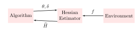
Figure 6.1: The interaction of a second-order stochastic gradient algorithm with an estimator that estimates the Hessian at the input point \(\theta\), with perturbation constant \(\delta\).
We first describe the classic FDSA scheme, which was proposed by (Fabian 1971). This scheme requires \(O(d^2)\) function observations to estimate the Hessian. Subsequently, we introduce the simultaneous perturbation trick to Hessian estimation and describe the following well-known variants that require a constant number of function observations, irrespective of the dimension \(d\):
- SPSA:
-
We consider two variants (both balanced) that require four and three function measurements, respectively;
- SF:
-
We present two variants that require one and two function measurements, respectively. Both methods are based on the idea of Gaussian smoothed functional, which was considered earlier in Chapter 3 in the context of gradient estimation;
- RDSA:
-
A scheme that requires three function measurements.
6.2 FDSA for Hessian estimation
Consider a scalar variable \(\theta\). A finite difference approximation of the first derivative for this simple case of a scalar parameter \(\theta\) is:
\[ \begin{align*} \frac{d f(\theta)}{d\theta} \approx \left(\dfrac{ f(\theta+\delta) - f(\theta-\delta)}{2\delta}\right). \tag{6.2} \end{align*} \]
Assuming the objective is smooth, and employing Taylor series expansions of \(f(\theta+\delta)\) and \(f(\theta-\delta)\) around \(\theta\), we obtain:
\[ \begin{align*} f(\theta\pm\delta) &= f(\theta) \pm \delta \frac{d f(\theta)}{d\theta} + \frac{\delta^2}{2} \frac{d^2 f(\theta)}{d\theta^2} + O(\delta^3), \\ \text{Thus, }\dfrac{ f(\theta+\delta) - f(\theta-\delta)}{2\delta} &= \dfrac{d f(\theta)}{d\theta} + O(\delta^2). \end{align*} \]
From the above, it is easy to see that the estimate (6.2) converges to the true gradient \(\dfrac{d f(\theta)}{d\theta}\) in the limit as \(\delta \rightarrow 0\).
This idea can be extended to estimate the second derivative by applying a finite difference approximation to the derivative in (6.2) as follows:
\[ \begin{align*} &\frac{d^2 f(\theta)}{d\theta^2} \approx \\ &\quad\frac{\left(\dfrac{ f(\theta+\delta + \delta) - f(\theta + \delta - \delta)}{2\delta}\right) - \left(\dfrac{ f(\theta - \delta + \delta) - f(\theta-\delta - \delta)}{2\delta}\right)}{2\delta} \tag{6.3} \end{align*} \]
As before, using Taylor series expansions, it can be shown that the RHS above is a good approximation to the second derivative.
For the case of a vector parameter, one needs to perturb each co-ordinate separately, leading to the following scheme for estimating the Hessian \(\nabla^2 f(\theta)\): For any \(i,j \in \{1,\ldots,d\}\),
\[ \begin{align*} \nabla^2_{ij} f(\theta) &\approx \frac{1}{4\delta^2}\bigg( f(\theta+\delta e_i + \delta e_j) + f(\theta+\delta e_i - \delta e_j) \\ &\qquad\qquad - \left( f(\theta-\delta e_i + \delta e_j) - f(\theta-\delta e_i - \delta e_j)\right)\bigg). \tag{6.4} \end{align*} \]
Such an approach requires \(4d^2\) number of function measurements to form the Hessian estimate. In the next section, we overcome this limitation by employing the simultaneous perturbation trick. Before that, we extend the estimate in (6.4) to the case of noisy function measurements. Suppose we have the following function measurements: For any \(i,j \in \{1,\ldots,d\}\),
\[ \begin{align*} &y^{++}_{ij} = f(\theta+\delta e_i + \delta e_j) + \xi^{++}_{ij}, \,\, y^{+-}_{ij} = f(\theta+\delta e_i - \delta e_j) + \xi^{+-}_{ij}, \tag{6.5} \\ &y^{-+}_{ij} = f(\theta-\delta e_i + \delta e_j) + \xi^{-+}_{ij} \textrm{ and } y^{--}_{ij} = f(\theta-\delta e_i - \delta e_j)+ \xi^{--}_{ij}. \tag{6.6} \end{align*} \]
Using these function measurements, we form the Hessian estimate \(\widehat H\) as follows:
\[ \begin{align*} \widehat H_{ij} & = \left(\dfrac{y^{++}_{ij} - y^{+-}_{ij} - y^{-+}_{ij} + y^{--}_{ij}}{4\delta^2}\right), \forall i,j \tag{6.7} \end{align*} \]
We analyze the bias of the estimator defined above, under the following assumptions:
Assumption A6.1.
\(f\) is four-times continuously differentiable1 with \(\left|\nabla^4_{i_1, i_2, i_3, i_4} f(\theta) \right| < \infty\), for \(i_1, i_2, i_3,i_4=1,\ldots, d\) and for all \(\theta\in \R^d\).
Assumption A6.2.
\(\E\left[\left. \xi^{++}_{ij} \right| \theta\right] = \E\left[\left. \xi^{+-}_{ij} \right| \theta\right] = \E\left[\left. \xi^{-+}_{ij} \right| \theta\right] = \E\left[\left. \xi^{--}_{ij} \right| \theta\right] = 0\) for \(i,j=1,\ldots,d\).
The four-times continuously differentiability assumption on \(f\) in A6.1 allows Taylor series expansions, while A6.2 ensures the noise factors vanish in the bias analysis. Under A6.1–A6.2, we have
\[ \begin{align*} \E[\widehat H_{ij} \mid \theta] &= \frac{1}{4\delta^2}\bigg( f(\theta+\delta e_i + \delta e_j) + f(\theta+\delta e_i - \delta e_j) \\ &\qquad\qquad - \left( f(\theta-\delta e_i + \delta e_j) - f(\theta-\delta e_i - \delta e_j)\right)\bigg) \\ & = \nabla^2_{ij} f(\theta) + O(\delta^2). \end{align*} \]
The final equality can be arrived at using Taylor series expansions followed by straightforward simplifications.
6.3 SPSA for Hessian estimation
6.3.1 Four measurements Hessian estimator
In this section, we present the Hessian estimation scheme from (J. C. Spall 2000). Let \(\Delta\) be a \(d\)-vector of symmetric, \(\pm 1\)-valued Bernoulli r.v.s, as in the case of first-order SPSA (see Section 3.2). Suppose \(G(\theta \pm \delta \Delta)\) are approximations to the gradient of \(f\) at \(\theta \pm \delta \Delta\). Then, the simultaneous perturbation trick suggests the following Hessian estimate:
\[ \begin{align*} \widehat H = \Delta^{-1}\dfrac{G(\theta + \delta \Delta) - G(\theta - \delta \Delta)}{4\delta}, \tag{6.8} \end{align*} \]
where \(\Delta^{-1} \stackrel{\triangle}{=} (1/\Delta_1,\ldots,1/\Delta_d)^T\).
What remains to be specified are the gradient estimates for input parameters \(\theta + \delta \Delta\). For forming this estimate, we use the simultaneous perturbation trick again, i.e.,
\[ G(\theta \pm \delta \Delta) = \hat\Delta^{-1}\dfrac{\left(y^{++} - y^+\right)}{\delta}, \]
where \(\hat \Delta\) denote a second independent set of perturbations having the same distribution as \(\Delta\),
\[ \begin{align*} & y^{++} = f(\theta + \delta \Delta + \delta \hat \Delta) + \xi^{++}, y^{-+} = f(\theta - \delta \Delta + \delta \hat \Delta) + \xi^{-+}, \\ & y^+ = f(\theta + \delta \Delta ) + \xi^{+},\textrm{ and } y^- = f(\theta - \delta \Delta) + \xi^{-}. \end{align*} \]
We can reuse these samples to form a SPSA-based gradient estimate as follows:
\[ \widehat \nabla f(\theta) = \Delta^{-1}\left(\frac{y^+ - y^-}{2\delta}\right). \]
We require the gradient as well as the Hessian estimates to implement a Newton step, as given in (6.1). The bias of the gradient estimate given above is analyzed in Chapter 3.
For the bias bound of the Hessian estimator defined in (6.8), we require the following assumption on the noise elements.
Assumption A6.3.
Let \(\Delta=(\Delta_1,\ldots,\Delta_d)\tr\) and \(\hat{\Delta}=(\hat\Delta_1,\ldots,\hat\Delta_d)\tr\) be two independent \(d\)-vectors of mutually independent, symmetric, \(\pm 1\)-valued Bernoulli r.v.s. Further, given \(\theta\), \(\{\xi^{++}, \xi^{-+}, \xi^{+}, \xi^{-}\}\) is independent of \(\Delta,\hat{\Delta}\). In addition,
\[ \E\left[\left. \xi^{++} \right| \theta\right] = \E\left[\left. \xi^{-+} \right| \theta\right] = \E\left[\left. \xi^{+} \right| \theta\right] = \E\left[\left. \xi^{-} \right| \theta\right] = 0. \]
Lemma 6.1.
Assume A6.1 and A6.3. Then, for any \(i,j \in \{1,\ldots, d\}\), we have
\[ \left| E\left[\left. \widehat H_{ij}\right |\theta \right] - \nabla_{i,j}^2 f(\theta) \right| = O(\delta^2), \]
where \(\widehat H_{ij}\) and \(\nabla^2_{i,j}f(\cdot)\) denote the \((i,j)\)th entry in the Hessian estimate \(\widehat H\) and the true Hessian \(\nabla^2 f(\cdot)\), respectively.
Proof.
Using A6.2, we have
\[ \begin{align*} E\left[\left. \widehat H_{ij}\right |\theta \right] &=E\Bigg[ \left[\frac{f(\theta+\delta\Delta+\delta{\hat{\Delta}}) -f(\theta+\delta\Delta)}{2\delta\Delta_i \delta {\hat{\Delta}}_j}\right] \\ & \qquad-\left .\left[\frac{f(\theta-\delta\Delta+\delta{\hat{\Delta}}) -f(\theta-\delta\Delta)}{2\delta\Delta_i \delta {\hat{\Delta}}_j}\right]\right |\, \theta \Bigg]. \tag{6.9} \end{align*} \]
Since \(f\) satisfies A6.1, we employ Taylor series expansions to obtain
\[ \begin{align*} f(\theta\pm\delta\Delta +\delta{\hat{\Delta}}) &= f(\theta\pm\delta\Delta) + \delta \sum_{k=1}^{d} {\hat{\Delta}}_k \nabla_k f(\theta\pm\delta\Delta) \\ &\quad+\frac{1}{2}\delta^2 \sum_{k=1}^{d} \sum_{l=1}^{d} {\hat{\Delta}}_k \nabla^2_{k,l} f(\theta \pm \delta\Delta) {\hat{\Delta}}_{l} +O(\delta^3). \end{align*} \]
Using (6.9) and the expansion above, we have
\[ \begin{align*} & E\left[\left. \widehat H_{ij}\right |\theta \right]= \\ & E \Bigg[ \frac{\nabla_i f(\theta+\delta\Delta) -\nabla_i f(\theta -\delta \Delta)}{2\delta\Delta_j} + \sum_{k\not= i} \frac{{\hat{\Delta}}_k}{{\hat{\Delta}}_i} \frac{\nabla_k f(\theta+\delta\Delta) -\nabla_k f(\theta -\delta \Delta)}{2\delta\Delta_j} \\ &+ \delta \sum_{k=1}^{d}\sum_{l=1}^{d} \frac{ {\hat{\Delta}}_k (\nabla^2_{k,l} f(\theta + \delta\Delta) - \nabla^2_{k,l} f(\theta - \delta\Delta)){\hat{\Delta}}_{l}}{4\delta\Delta_j {\hat{\Delta}}_i} + O(\delta^2) \hspace{6pt}|\hspace{6pt} \theta\Bigg] \tag{6.10} \end{align*} \]
Expanding \(\nabla_if(\theta\pm\delta\Delta)\) around \(\nabla_if(\theta)\), we obtain
\[ \frac{\nabla_i f(\theta+\delta\Delta) -\nabla_i f(\theta -\delta \Delta)}{2\delta\Delta_j} = \nabla_{i,j}^2f(\theta) + \sum_{l \not= j} \frac{\Delta_l}{\Delta_j} \nabla_{l,j}^2f(\theta) + O(\delta^3). \]
The second term on the RHS of (6.10) can be simplified in an analogous fashion.
The third term on the RHS of of (6.10) can be simplified as follows:
\[ \begin{align*} & \delta \sum_{k=1}^{d}\sum_{l=1}^{d} \frac{ {\hat{\Delta}}_k (\nabla^2_{k,l} f(\theta + \delta\Delta) - \nabla^2_{k,l} f(\theta - \delta\Delta)) {\hat{\Delta}}_l}{ 4\delta\Delta_j {\hat{\Delta}}_i} \\ & =\delta \sum_{k=1}^{d}\sum_{l=1}^{d} \sum_{m=1}^{d} \frac{{\hat{\Delta}}_k \Delta(m) \nabla^3_{k,l,m} f(\theta) {\hat{\Delta}}_l}{2{\hat{\Delta}}_i\Delta_j} + O(\delta^2). \end{align*} \]
In the above, we used the following equality:
\[ \frac{\nabla^2_{k,l}f(\theta+\delta\Delta) - \nabla^2_{k,l}f(\theta-\delta\Delta)}{4\delta\Delta_j} = \sum_{m=1}^{d} \frac{\Delta(m)\nabla^3_{k,l,m}f(\theta)}{2\Delta_j} +O(\delta^2) \]
Using the simplified forms for each of the terms on the RHS of (6.10), we have
\[ \begin{align*} & E\left[\left. \widehat H_{ij}\right |\theta \right] = E \Bigg[\nabla_{i,j}^2f(\theta) +\sum_{l\not= i} \frac{\Delta_l}{\Delta_i} \nabla_{i,l}^2f(\theta) +\sum_{k\not= j} \frac{{\hat{\Delta}}_k}{{\hat{\Delta}}_j} \nabla_{k,i}^2f(\theta) \\ &\qquad+ \sum_{k\not= i}\sum_{l\not= i} \frac{{\hat{\Delta}}_k}{{\hat{\Delta}}_i} \frac{\Delta_l}{\Delta_j} \nabla_{k,l}^2f(\theta) + \delta \sum_{k,l,m=1}^{d} \frac{{\hat{\Delta}}_k \Delta(m) \nabla^3_{k,l,m} f(\theta) {\hat{\Delta}}_l}{2{\hat{\Delta}}_i\Delta_j} +O(\delta^2) \hspace{3pt}|\hspace{3pt} \theta\Bigg] \\ &= \nabla_{i,j}^2f(\theta) + \sum_{l\not= j} E\left [\frac{\Delta_l}{\Delta_j} \hspace{3pt}|\hspace{3pt} \theta \right] \nabla_{i,l}^2f(\theta) + \sum_{k\not= i} E\left [\frac{{\hat{\Delta}}_k}{{\hat{\Delta}}_i} \hspace{3pt}|\hspace{3pt} \theta\right] \nabla_{k,i}^2f(\theta) \\ &+ \sum_{k\not= i}\sum_{l\not= j}E\left[\left.\frac{{\hat{\Delta}}_k}{{\hat{\Delta}}_i} \frac{\Delta_l}{\Delta_j} \hspace{3pt}\right|\hspace{3pt} \theta\right] \nabla_{k,l}^2f(\theta) \\ &\qquad\qquad\qquad+ \delta \sum_{k=1}^{d}\sum_{l=1}^{d}\sum_{m=1}^{d} E\left[\left.\frac{ {\hat{\Delta}}_k{\hat{\Delta}}_l \Delta(m)}{ 2{\hat{\Delta}}_j\Delta_i} \hspace{3pt}\right|\hspace{3pt} \theta\right] \nabla^3_{k,l,m}f(\theta) + O(\delta^2). \end{align*} \]
Since \(\Delta, \hat\Delta\) are independent vectors of zero mean, symmetric Bernoulli r.v.s, each term involving an expectation on the RHS above vanishes. The claim follows.
\(\square\)
6.3.2 Three measurements Hessian estimator
We now present a variation to 2SPSA, where the number of function measurements required for forming the Hessian estimate is brought down to three. This scheme was proposed by (Bhatnagar and Prashanth 2015), and can be motivated by using the following balanced approximation to the second derivative in the case of a scalar parameter:
\[ \begin{align*} \frac{d^2 f(\theta)}{d\theta^2} \approx \frac{\left(\dfrac{ f(\theta+\delta) - f(\theta)}{\delta}\right) - \left(\dfrac{ f(\theta) - f(\theta-\delta)}{\delta}\right)}{\delta} \\ = \left(\dfrac{ f(\theta+\delta) + f(\theta-\delta) - 2 f(\theta)}{\delta^2}\right). \tag{6.11} \end{align*} \]
The extension to a vector parameter is performed by using the following function measurements:
\[ y^{++} = f(\theta+\delta \Delta + \delta \hat\Delta) + \xi^{++}, y^{--} = f(\theta-\delta \Delta - \delta\hat\Delta) + \xi^{--}, \textrm{ and }y = f(\theta)+ \xi. \]
Using \(y^{\pm}\) and \(y\), together with two random perturbation vectors \(\Delta\) and \(\hat \Delta\) (as in the previous section), the Hessian estimate \(\widehat H\) is formed as follows:
\[ \begin{align*} \widehat H_{ij} = \left(\dfrac{y^{++} + y^{--} - 2 y}{\delta^2 \Delta_i \hat \Delta_j}\right), \forall i,j. \tag{6.12} \end{align*} \]
Reusing the sample measurements, we form the gradient estimate as follows:
\[ \widehat\nabla f(\theta) = \Delta^{-1}\frac{y^{++}-y^{--}}{2\delta}. \]
For the noise elements to vanish in the bias analysis of the Hessian estimator above, we make the following assumption.
Assumption A6.4.
Let \(\Delta=(\Delta_1,\ldots,\Delta_d)^T\) and \(\hat{\Delta}=(\hat\Delta_1,\ldots,\hat\Delta_d)\tr\) be two independent \(d\)-vectors of mutually independent, symmetric, \(\pm 1\)-valued Bernoulli r.v.s. Further, given \(\theta\), \(\{\xi, \xi^{++},\xi^{--}\}\) is independent of \(\Delta, \hat\Delta\). In addition,
\(\E\left[\left. \xi^{++} \right| \theta\right] = \E\left[\left. \xi^{--} \right| \theta\right] = \E\left[\left. \xi \right| \theta\right] = 0\).
Proof.
We first consider the case when \(i,j\in\{1,\ldots,d\}\), \(i\not=j\). Let
\[ \hat{f}(\theta,\Delta,\hat{\Delta})=f(\theta+\delta \Delta + \delta \hat\Delta) + f(\theta-\delta \Delta - \delta \hat\Delta) - 2 f(\theta). \]
Then, using suitable Taylor’s expansions, we obtain
\[ \begin{align*} \frac{\hat{f}(\theta,\Delta,\hat{\Delta})}{\delta^2 \Delta_i\hat{\Delta}_j} &= \frac{(\Delta+\hat{\Delta})^T \nabla^2 f(\theta)(\Delta +\hat{\Delta})}{\Delta_i\hat{\Delta}_j} + O(\delta^2) \\ &= \sum_{l=1}^{d}\sum_{m=1}^{d} \frac{\Delta_l\nabla^2_{lm}f(\theta)\Delta_m}{\Delta_i \hat{\Delta}_j} + 2\sum_{l=1}^{d}\sum_{m=1}^{d} \frac{\Delta_l\nabla^2_{lm} f(\theta)\hat{\Delta}_m}{\Delta_i \hat{\Delta}_j} \\ &\qquad+ \sum_{l=1}^{d}\sum_{m=1}^{d} \frac{\hat{\Delta}_l\nabla^2_{lm}f(\theta)\hat{\Delta}_m}{\Delta_i \hat{\Delta}_j} + O(\delta^2). \end{align*} \]
It is now easy to see that
\[ \begin{align*} &\E\left[\sum_{l=1}^{d}\sum_{m=1}^{d}\left. \frac{\Delta_l\nabla^2_{lm}f(\theta)\Delta_m}{\Delta_i \hat{\Delta}_j}\right| \theta\right] \\ & = \E\left[\sum_{l=1}^{d}\sum_{m=1}^{d}\left. \frac{\hat{\Delta}_l\nabla^2_{lm}f(\theta)\hat{\Delta}_m}{\Delta_i \hat{\Delta}_j}\right| \theta\right] = 0 \mbox{ a.s., and } \\ & \E\left[\sum_{l=1}^{d}\sum_{m=1}^{d} \frac{\Delta_l\nabla^2_{lm}f(\theta)\hat{\Delta}_m}{\Delta_i \hat{\Delta}_j}\mid \theta\right] = \nabla_{i,j}^2f(\theta) \mbox{ a.s.} \end{align*} \]
Thus,
\[ \E\left[\left. \frac{\hat{f}(\theta, \Delta, \hat{\Delta})}{\delta^2 \Delta_i\hat{\Delta}_j} \right| \theta \right] = 2\nabla_{i,j}^2f(\theta) + O(\delta^2). \]
The case when \(i=j\in\{1,\ldots,d\}\) follows in a similar manner. The claim follows after observing that
\[ \E\left[ \left.\widehat H_{ij} \right| \theta\right]= \E\left[\left. \frac{\hat{f}(\theta, \Delta, \hat{\Delta})}{\delta^2 \Delta_i\hat{\Delta}_j} \right| \theta \right]. \]
The equality above holds since the noise elements \(\xi^{++}, \xi^{--}, \xi\) satisfy A6.4.
\(\square\)
6.4 Gaussian smoothed functional for Hessian estimation
We now present a couple of Hessian estimation procedures from (Bhatnagar 2007) that are based on Gaussian smoothing.
6.4.1 One-Measurement SF (1SF) Estimator
We begin with a one-measurement Hessian estimator \(D_{\delta,1}^2f(\theta)\) that uses one function measurement with the same perturbed parameter as the one-measurement gradient SF procedure. We shall later provide a two-sided Hessian estimator as well that estimates both the Hessian and the gradient using two function measurements. We shall continue to assume A6.1.
As with gradient SF, we begin by taking a convolution of the objective function Hessian with a multi-variate Gaussian density functional. Through an integration-by-parts argument applied twice, the same is seen to be a convolution of the objective function with a scaled Gaussian density functional. Let
\[ D_{\delta, 1}^2 f(\theta) = \int G_{\delta}(\theta - \Delta') \nabla^2_{\Delta'} f(\Delta') d \Delta', \tag{6.13} \]
denote the convolution of the Hessian \(\nabla^2_{\Delta'} f(\Delta')\) with the \(d\)-dimensional multivariate normal p.d.f.
\[ G_{\delta}(\theta-\Delta') = \frac{1}{(2\pi)^{d/2}\delta^d} \exp \left( -\frac{1}{2}\sum_{i=1}^{d} \frac{(\theta_i-\Delta'_i)^2}{\delta^2} \right), \]
where \(\theta, \Delta' \in {\cal R}^d\).
Assumption A6.5.
Let \(\Delta=(\Delta_1,\ldots,\Delta_d)^T\) where \(\Delta_i\sim N(0,1)\), \(i=1,\ldots,d\) and with \(\Delta_i\) independent of \(\Delta_j\), \(\forall i\not=j\). Further, given \(\theta\), \(\xi^+\) is independent of \(\Delta\). Further, \(\E\left[\left. \xi^+ \right| \theta\right] = 0\).
Let \(y^+=f(\theta+\delta\Delta)+\xi^+\) denote a noisy function measurement, where \(\xi^+\) denotes the measurement noise. The one-simulation (1SF) Hessian estimator is then the following:
\[ \begin{align*} \hat{H}(\theta) = \frac{(\Delta\Delta\tr-I)}{\delta^2} y^+. \tag{6.14} \end{align*} \]
The reason for having this form for the Hessian estimator will become evident in Proposition 6.1.
As with earlier estimates, we can reuse the function measurement \(y^+\) to form a gradient estimate as follows:
\[ \widehat \nabla f(\theta)=\Delta\left(\frac{y^+}{\delta}\right). \]
Proposition 6.1 (Stein’s Lemma for Hessian Estimation).
\[ D_{\delta, 1}^2 f(\theta) =\frac{1}{\delta^2} E \left[ (\Delta{\Delta}^T - I) f(\theta +\delta \Delta)\right], \]
where the expectation above is taken w.r.t. the \(d\)-dimensional multivariate normal p.d.f. \(G(\Delta)\) corresponding to the random vector of \(d\) independent \(N(0,1)\)–distributed random variables.
Proof.
Upon integrating by parts, one obtains
\[ D_{\delta, 1}^2 f(\theta) = \int \nabla_{\theta} G_{\delta}(\theta - \Delta') \nabla_{\Delta'} f(\Delta') d \Delta'. \tag{6.15} \]
Now
\[ \nabla_{\theta} G_{\delta}(\theta - \Delta') = -\frac{(\theta - \Delta')}{\delta^2} G_{\delta}(\theta - \Delta'). \]
Upon substituting the above in (6.15) and performing integration-by-parts, we obtain
\[ D_{\delta, 1}^2 f(\theta) =-\frac{1}{\delta^2} \int \nabla_{\theta}((\theta - \Delta')G_{\delta}(\theta - \Delta')) f(\Delta') d \Delta'. \]
A change of variables then gives
\[ D_{\delta, 1}^2 f(\theta) = -\frac{1}{\delta^2} \int \nabla_{\Delta'}(\Delta' G_{\delta}(\Delta')) f(\theta - \Delta') d \Delta'. \tag{6.16} \]
We now evaluate \(\nabla_{\Delta'}(\Delta' G_\delta(\Delta'))\) \(=\nabla_{\Delta'}((\Delta'_1G_\delta(\Delta'),\ldots\), \(\Delta'_NG_\delta(\Delta'))\). Note that
\[ \nabla_{\Delta'}(\Delta' G_\delta(\Delta'))= \]
\[ \left[ \begin{array}{cccc} \nabla_{\Delta'_1}(\Delta'_1 G_\delta(\Delta')) & \nabla_{\Delta'_2}(\Delta'_1 G_\delta(\Delta')) & \cdots & \nabla_{\Delta'_d}(\Delta'_1 G_\delta(\Delta')) \\ \nabla_{\Delta'_1}(\Delta'_2 G_\delta(\Delta')) & \nabla_{\Delta'_2}(\Delta'_2 G_\delta(\Delta')) &\cdots & \nabla_{\Delta'_d}(\Delta'_2 G_\delta(\Delta')) \\ \cdots & \cdots & \cdots &\cdots \\ \nabla_{\Delta'_1}(\Delta'_d G_\delta(\Delta')) & \nabla_{\Delta'_2}(\Delta'_d G_\delta(\Delta')) & \cdots & \nabla_{\Delta'_d}(\Delta'_d G_\delta(\Delta')) \end{array} \right] \]
\[ =\left[ \begin{array}{cccc} \left(1-\frac{{\Delta'}_1^2}{\delta^2}\right) & -\frac{\Delta'_1\Delta'_2}{\delta^2} & \cdots & -\frac{\Delta'_1\Delta'_d}{\delta^2}\\ -\frac{{\Delta'}_2\Delta'_1}{\delta^2} & \left(1-\frac{{\Delta'}_2^2}{\delta^2}\right) & \cdots & -\frac{\Delta'_2\Delta'_d}{\delta^2}\\ \cdots & \cdots & \cdots & \cdots \\ -\frac{\Delta'_d\Delta'_1}{\delta^2} & -\frac{\Delta'_d\Delta'_2}{\delta^2} & \cdots & \left(1-\frac{{\Delta'}_d^2}{\delta^2}\right) \end{array} \right]G_{\delta}(\Delta') \]
\[ = \left(I - \frac{\Delta'{\Delta'}^T}{\delta^2}\right) G_\delta(\Delta') \stackrel{\triangle}{=} \check{H}(\Delta') G_\delta(\Delta'). \]
From (6.16), we have
\[ D_{\delta, 1}^2 f(\theta) = -\frac{1}{\delta^2} \int \check{H}(\Delta') G_{\delta}(\Delta') f(\theta-\Delta') d \Delta'. \]
Let \(\Delta \stackrel{\triangle}{=} \Delta'/\delta\). Then \(d\Delta' = \delta^d d \Delta\). From (6.16), we then obtain
\[ D_{\delta, 1}^2 f(\theta) = \frac{1}{\delta^2} \int \bar{I}(\Delta) \left(\frac{1}{(2\pi)^{d/2}} \exp(-\frac{1}{2}\sum_{i=1}^{d}(\Delta_{i})^{2})\right) f(\theta -\delta\Delta) d\Delta, \tag{6.17} \]
where
\[ \bar{I}(\Delta) \stackrel{\triangle}{=} (\Delta{\Delta}^T - I). \tag{6.18} \]
Note that \(\Delta_i\), \(i=1,\ldots, d\) are independent \(N(0,1)\) distributed random variables. Now since \(\Delta\) and \(-\Delta\) have the same distribution, one obtains
\[ D_{\delta, 1}^2 f(\theta) =\frac{1}{\delta^2} E \left[ (\Delta{\Delta}^T - I) f(\theta +\delta \Delta)\right]. \]
The claim follows.
\(\square\)
Proof.
From the definition of \(\hat{H}(\theta)\),
\[ E[\hat{H}(\theta)|\theta)] = \frac{1}{\delta^2}E[\bar{I}(\Delta) (f(\theta+\delta\Delta)+\xi^+)|\theta] \]
\[ = D_{\delta,1}^2 f(\theta) + \frac{1}{\delta^2} E[(I-\Delta\Delta\tr)\xi^+|\theta]. \]
The second term on the RHS equals zero in the light of Assumption A6.5. Now, from Proposition 6.1, we have that
\[ D_{\delta,1}^{2} f(\theta) = \E\left[\frac{1}{\delta^2}\bar{I}(\Delta) f(\theta+\delta \Delta) \mid \theta \right], \]
where \(\Delta = (\Delta_1,\ldots, \Delta_d)^T\) is a vector of independent \(N(0,1)\) random variates and the expectation is taken w.r.t. the density of \(\Delta\). Using a Taylor series expansion of \(f(\theta + \delta \Delta)\) around \(\theta\), one obtains
\[ \begin{array}{ll} D_{\delta,1}^2 f(\theta) & = E\bigg[\dfrac{1}{\delta^2} \bar{I}(\Delta) (f(\theta) + \delta \Delta\tr \nabla f(\theta) \\ & \qquad\qquad\qquad+ \dfrac{\delta^2}{2}\Delta\tr \nabla^2 f(\theta) \Delta + o(\delta^2) \mid \theta \bigg] \\ & = \dfrac{1}{\delta^2} E[\bar{I}(\Delta) f(\theta)\mid \theta] + \dfrac{1}{\delta} E[\bar{I}(\Delta)\Delta\tr \nabla f(\theta)\mid \theta] \\ & \qquad\qquad\qquad+ \frac{1}{2}E[ \bar{I}(\Delta) \Delta\tr \nabla^2f(\theta) \Delta\mid \theta] + O(\delta). \end{array} \tag{6.19} \]
Now observe that \(E[\bar{I}(\Delta)] =0\) (the matrix of all zero elements) with \(E[\bar{H}(\Delta)]\). Hence the first term on the RHS of (6.19) equals zero. Now consider the second term on the RHS of (6.19). Note that
\[ \begin{array}{l} E[\bar{I}(\Delta)\Delta\tr\nabla f(\theta)\mid\theta] = \\ \E\left[ $\begin{array}{@{\hspace{2ex}}c@{\hspace{2ex}}c@{\hspace{2ex}}c@{\hspace{2ex}}c} (\Delta_{1}^{2}-1)\Delta\tr\nabla f(\theta) & \Delta_1\Delta_2\Delta\tr\nabla f(\theta) & \cdots & \Delta_1\Delta_d\Delta\tr\nabla f(\theta)\\[1ex] \Delta_2\Delta_1\Delta\tr\nabla f(\theta) & (\Delta_{2}^{2}-1)\Delta\tr\nabla f(\theta) & \cdots & \Delta_2\Delta_d\Delta\tr\nabla f(\theta)\\[1ex] \cdots & \cdots & \cdots & \cdots \\[1ex] \Delta_d\Delta_1\Delta\tr\nabla f(\theta) & \Delta_d\Delta_2\Delta\tr\nabla f(\theta) & \cdots & (\Delta_{d}^{2}-1)\Delta\tr\nabla f(\theta) \end{array}$ \mid \theta \right]. \end{array} \tag{6.20} \]
One can verify that expectation of each term (conditioned on \(\theta\)) within the matrix above equals zero since \(E[\Delta_i]=\E[\Delta_i^3]=0\) and \(\E[\Delta_i^2]=1\), \(\forall i=1,\ldots,d\). Also, \(\Delta_i\) is independent of \(\Delta_j\) for all \(i\not= j\). Hence the second term on the RHS of (6.19) equals zero as well. Consider now the third term on the RHS of (6.19). Note that
\[ \frac{1}{2}\E[\bar{H}(\Delta)\Delta\tr\nabla^2 f(\theta)\Delta\mid \theta] = \]
\[ \frac{1}{2}\E\left[ $\begin{array}{@{\hspace{2ex}}c@{\hspace{2ex}}c@{\hspace{2ex}}c} (\Delta_{1}^{2}-1)\sum\limits_{i,j=1}^{d}\nabla_{ij}f(\theta)\Delta_i\Delta_j & \cdots & \Delta_1\Delta_d\sum\limits_{i,j=1}^{d}\nabla_{ij}f(\theta)\Delta_i\Delta_j\\[2ex] \Delta_2\Delta_1\sum\limits_{i,j=1}^{d}\nabla_{ij}f(\theta)\Delta_i\Delta_j & \cdots & \Delta_2\Delta_d\sum\limits_{i,j=1}^{d}\nabla_{ij}f(\theta)\Delta_i\Delta_j\\[2ex] \cdots & \cdots & \cdots \\[2ex] \Delta_d\Delta_1\sum\limits_{i,j=1}^{d}\nabla_{ij}f(\theta)\Delta_i\Delta_j & \cdots & (\Delta_{d}^{2}-1)\sum\limits_{i,j=1}^{d}\nabla_{ij}f(\theta)\Delta_i\Delta_j \end{array}$ \mid \theta \right]. \tag{6.21} \]
Consider now the term corresponding to the first row and first column above. Note that
\[ \begin{array}{l} \E[(\Delta_{1}^{2}-1)\sum_{i,j=1}^{d}\nabla_{ij}f(\theta)\Delta_i\Delta_j\mid \theta]\\ = \E[\Delta_{1}^{2}\sum_{i,j=1}^{d}\nabla_{ij}f(\theta)\Delta_i\Delta_j\mid \theta] - \E[\sum_{i,j=1}^{d}\nabla_{ij}f(\theta)\Delta_i\Delta_j\mid \theta]. \end{array} \tag{6.22} \]
The first term on the RHS of (6.22) equals
\[ \begin{array}{l} \E[\Delta_1^4\nabla_{11}f(\theta)\mid \theta] + \E[\sum_{i=j,i\not=1} \Delta_1^2\Delta_i^2\nabla_{ij}f(\theta)\mid \theta] \\[1ex] + \E[\sum_{i\not=j,i\not=1}\Delta_1^2\Delta_i\Delta_j\nabla_{ij}f(\theta)\mid \theta] = 3\nabla_{11}f(\theta) +\sum_{i=j,i\not=1}\nabla_{ij}f(\theta), \end{array} \]
since \(\E[\Delta_1^4] =3\). The second term on RHS of (6.22) equals \({\displaystyle -\sum_{i=1}^{d}\nabla_{ii}f(\theta)}\). Adding the above two terms, one obtains
\[ \E[(\Delta_{1}^{2}-1)\sum_{i,j=1}^{d}\nabla_{ij}f(\theta)\Delta_i\Delta_j\mid \theta] = 2\nabla_{11}f(\theta). \]
Consider now the term in the first row and second column of the matrix in (6.21). Note that
\[ \begin{array}{l} \E[\Delta_1\Delta_2\sum_{i,j=1}^{d}\nabla_{ij}f(\theta)\Delta_i\Delta_j\mid \theta]\\[1ex] =2\E[\Delta_1^2\Delta_2^2\nabla_{12}f(\theta)\mid \theta] + \E[\sum_{(i,j)\not\in \{(1,2),(2,1)\}} \Delta_1\Delta_2\Delta_i\Delta_j \nabla_{ij}f(\theta)\mid \theta] \\[1ex] = 2\nabla_{12}f(\theta). \end{array} \]
Proceeding in a similar manner, it is easy to verify that the \((i,j)\)th term (\(i,j\in \{1,\ldots, d\}\)) in the matrix in (6.21) equals \(2\nabla_{ij}f(\theta)\). Substituting the above back in (6.21), one obtains
\[ \frac{1}{2}\E[\bar{I}(\Delta)\Delta\tr\nabla^2 f(\theta)\Delta] = \nabla^2 f(\theta). \]
Thus, (6.19) now becomes
\[ D^2_{\delta,1} f(\theta) = \nabla^2 f(\theta) + O(\delta). \]
The claim follows.
\(\square\)
6.4.2 Two-measurement SF (2SF) estimator
We now present the balanced form of the Hessian estimator from (Bhatnagar 2007) that requires only two function measurements. Let
\[ D_{\delta, 2}^2 f(\theta) = E \left[\frac{1}{2\delta^2} \bar{I}(\Delta) (f(\theta +\delta \Delta) + f(\theta -\delta \Delta)) \mid \theta\right], \]
with \(\bar{I}(\Delta)\) as in (6.18). We now present the balanced form of the Hessian estimator based on two function measurements. Let \(y^+=f(\theta+\delta\Delta)+\xi^+\) and \(y^-=f(\theta+\delta\Delta)+\xi^-\), respectively, where \(\xi^+\) and \(\xi^-\) denote the measurement noise in \(y^+\) and \(y^-\). The 2SF Hessian estimator is then the following:
\[ \begin{align*} \hat{H}(\theta) = \frac{(\Delta\Delta\tr-I)}{2\delta^2} (y^++y^-). \tag{6.23} \end{align*} \]
A gradient estimate re-using the function measurements \(y^\pm\) is given by
\[ \widehat\nabla f(\theta)=\Delta\left(\frac{y^+-y^-}{2\delta}.\right) \]
This gradient estimate’s bias was analyzed earlier in Chapter 3. We analyze the bias of the Hessian estimator in (6.23). For this analysis, we shall continue to assume A6.1. In addition, we have the following assumption on the measurement noise:
Assumption A6.6.
Let \(\Delta=(\Delta_1,\ldots,\Delta_d)^T\) where \(\Delta_i\sim N(0,1)\), \(i=1,\ldots,d\) and with \(\Delta_i\) independent of \(\Delta_j\), \(\forall i\not=j\). Further, given \(\theta\), \(\xi^+\) and \(\xi^-\) are independent of \(\Delta\) and they are also independent of each other. Further, \(\E\left[\left. \xi^+ \right| \theta\right] = \E\left[\left. \xi^- \right| \theta\right] = 0\).
Proof.
From (6.23), note that
\[ E[\hat{H}(\theta)|\theta)] = \frac{1}{2\delta^2}E[\bar{I}(\Delta) ((f(\theta+\delta\Delta)+\xi^+)+(f(\theta-\delta\Delta)+\xi^-)|\theta] \]
\[ = D_{\delta,2}^2 f(\theta) + \frac{1}{2\delta^2} E[(I-\Delta\Delta\tr)(\xi^++\xi^-)|\theta]. \]
The second term on the RHS equals zero in the light of Assumption A6.6.
We now consider the first term on the RHS above. Using Taylor series expansions of \(f(\theta +\delta\Delta)\) and \(f(\theta -\delta\Delta)\) around \(\theta\), one obtains
\[ f(\theta+\delta \Delta) = f(\theta) + \delta \Delta\tr \nabla f(\theta) + \frac{\delta^2}{2}\Delta\tr \nabla^2 f(\theta) \Delta + \frac{\delta^3}{6} \nabla^3 f(\theta) (\Delta \otimes \Delta \otimes \Delta) + O(\delta^4) \]
\[ f(\theta-\delta \Delta) = f(\theta) - \delta \Delta\tr \nabla f(\theta) + \frac{\delta^2}{2}\Delta\tr \nabla^2 f(\theta) \Delta - \frac{\delta^3}{6} \nabla^3 f(\theta) (\Delta \otimes \Delta \otimes \Delta) + O(\delta^4). \]
From the foregoing, one obtains
\[ D_{\delta, 2}^2 f(\theta) = E \left[\frac{1}{2\delta^2} \bar{I}(\Delta) \left(2f(\theta) + \delta^2 \Delta\tr\nabla^2 f(\theta)\Delta +O(\delta^4)\right)\mid \theta\right]. \]
It has been shown in the proof of Proposition 6.2 that \(\E[\bar{I}(\Delta) f(\theta)\mid\theta]=0\) and \({\displaystyle \frac{1}{2} \E[\bar{I}(\Delta) \Delta\tr \nabla^2 f(\theta) \Delta\mid\theta] = \nabla^2 J(\theta)}\), respectively. We thus have
\[ D^2_{\delta,2} f(\theta) = \nabla^2 f(\theta) + O(\delta^2). \]
The claim follows.
\(\square\)
6.5 RDSA for Hessian estimation
In this section, the random perturbations are chosen using an asymmetric Bernoulli distribution. More precisely, we choose \(\Delta_i\), \(i=1,\ldots,d\), i.i.d. as follows:
\[ \Delta_i = \begin{cases} -1 & \text{ w.p. } \dfrac{(1+\epsilon)}{(2+\epsilon)}, \\ 1+\epsilon & \text{ w.p. } \dfrac{1}{(2+\epsilon)}, \end{cases} \tag{6.24} \]
where \(\epsilon>0\) is a constant that can be chosen to be arbitrarily small. Note that, for any \(i=1,\ldots,d\), \(\E \Delta_i = 0\), \(\E (\Delta_i)^2 = 1+\epsilon\) and \(\E (\Delta_i)^4 = \dfrac{(1+\epsilon)(1+(1+\epsilon)^3)}{(2+\epsilon)}\). Henceforth, we will use \(\tau\) to denote \(E (\Delta_i)^4\).
Suppose we have the following function measurements:
\[ y^+ = f(\theta+\delta \Delta) + \xi^+, y^- = f(\theta-\delta \Delta)+ \xi^-, \textrm{ and }y = f(\theta)+ \xi. \]
We would like to obtain a Hessian estimate \(\widehat H\) that is not too far from the true Hessian \(\nabla^2 f(\theta)\). Suppose we use the three measurements above, together with a matrix \(M\) (to be specified later) to form \(\widehat H\) as follows:
\[ \begin{align*} \widehat H & = M \left(\dfrac{y^+ + y^- - 2 y}{\delta^2}\right) \tag{6.25} \\ & = M \left[\left(\dfrac{f(\theta+\delta \Delta) + f(\theta-\delta \Delta) - 2 f(\theta)}{\delta^2}\right) + \left(\dfrac{\xi^+ + \xi^- - 2 \xi}{\delta^2}\right)\right] \\ & = M \left(\Delta\tr \nabla^2 f(\theta) \Delta + O(\delta^2) + \left(\dfrac{\xi^+ + \xi^- - 2 \xi}{\delta^2} \right)\right). \tag{6.26} \end{align*} \]
We form a gradient estimate using \(y^\pm\) as follows:
\[ \widehat\nabla f(\theta)= \frac{1}{(1+\epsilon)}\Delta \left(\frac{y^+-y^-}{2\delta}\right). \]
The bias of this estimator is analyzed in Chapter 3.
We now deconstruct the Hessian estimate in (6.26). Taking expectations on both sides of (6.26), we observe that the last term in (6.26) vanishes, while the first and second term remain. However, we do not have the true Hessian in the first term and it would be nice to recover \(\nabla^2 f(\theta)\) from this term via a suitable matrix \(M\) and the following definition for \(M\) achieves this goal:
\[ \begin{align*} M = \left[ \begin{array}{ccc} \frac{1}{\kappa}\left((\Delta_1)^2\!-(1+\epsilon)\right) & \cdots & \frac{1}{2(1+\epsilon)^2}\Delta_1 \Delta_d\\ \frac{1}{2(1+\epsilon)^2}\Delta_2 \Delta_1 & \cdots & \frac{1}{2(1+\epsilon)^2}\Delta_2 \Delta_d\\ \cdots&\cdots&\cdots\\ \frac{1}{2(1+\epsilon)^2}\Delta_d \Delta_1 & \cdots & \frac{1}{\kappa}\left((\Delta_d)^2-(1+\epsilon)\right) \\ \end{array} \right], \tag{6.27} \end{align*} \]
where \(\kappa = \tau \left(1- \dfrac{(1+\epsilon)^2}{\tau}\right)\) and \(\tau = E (\Delta_i)^4= \dfrac{(1+\epsilon)(1+(1+\epsilon)^3)}{(2+\epsilon)}\), for any \(i=1,\ldots, d\).
While the definition of \(M\) above looks complicated, the motivation behind such a definition can be seen through the following calculation that established that the first term, i.e., \(M \left(\Delta\tr \nabla^2 f(\theta) \Delta\right)\) in (6.26) turns out to be the true Hessian evaluated at \(\theta\).
As before, we make the following assumption to ensure noise elements vanish in the analysis of the RDSA Hessian estimator (6.25).
Assumption A6.7.
Let \(\Delta=(\Delta_1,\ldots,\Delta_d)^T\) be a \(d\)-vector of mutually independent, asymmetric, Bernoulli r.v.s satisfying (6.24). Further, given \(\theta\), \(\{\xi, \xi^+,\xi^-\}\) is independent of \(\Delta\). In addition, \(\E\left[\left. \xi^+ \right| \theta\right] = \E\left[\left. \xi^- \right| \theta\right] = \E\left[\left. \xi \right| \theta\right] = 0\).
Lemma 6.3.
(Bias in Hessian estimate) Assume A6.1 and A6.7. Then, \(\widehat H\) defined according to (6.27) satisfies the following bound for any \(i,j = 1,\ldots, d\),
\[ \begin{align*} \left|\E\left[ \left. \widehat H(i,j) \right| \theta \right] - \nabla^2_{ij} f(\theta)\right| = O(\delta^2). \tag{6.28} \end{align*} \]
From the above lemma, it is evident that the bias in the Hessian estimate above is of the same order as that of the other balanced estimators in the previous sections.
Proof.
By a Taylor’s expansion, we obtain
\[ \begin{align*} &f(\theta \pm \delta \Delta) = f(\theta) \pm \delta \Delta\tr \nabla f(\theta) + \frac{\delta^2}{2} \Delta\tr \nabla^2 f(\theta) \Delta \\ &\pm \frac{\delta^3}{6} \nabla^3 f(\theta) (\Delta \otimes \Delta \otimes \Delta) + \frac{\delta^4}{24} \nabla^4 f(\tilde \theta^+)(\Delta \otimes \Delta \otimes \Delta \otimes \Delta). \end{align*} \]
Hence,
\[ \begin{align*} &\dfrac{f(\theta+\delta \Delta) + f(\theta-\delta \Delta) - 2 f(\theta)}{\delta^2} \\ =& \Delta\tr \nabla^2 f(\theta) \Delta + O(\delta^2) \\ = & \sum\limits_{i=1}^d\sum\limits_{j=1}^d \Delta_i \Delta_j \nabla^2_{ij} f(\theta) + O(\delta^2) \\ =& \sum\limits_{i=1}^d (\Delta_i)^2 \nabla^2_{ii} f(\theta) + 2\sum\limits_{i=1}^{d-1}\sum\limits_{j=i+1}^d \Delta_i \Delta_j \nabla^2_{ij} f(\theta) + O(\delta^2). \end{align*} \]
Now, taking the conditional expectation of the Hessian estimate \(\widehat{H}\) and observing that \(\E[\xi^+ + \xi^- - 2\xi \mid \theta] = 0\) by A6.7, we obtain the following:
\[ \begin{align*} \E[\widehat H \mid \theta] = & \E\left[\left. M \left(\sum\limits_{i=1}^{d-1} (\Delta_i)^2 \nabla^2_{ii} f(\theta) \right.\right.\right. \\ &\left.\left.\left.+ 2\sum\limits_{i=1}^d\sum\limits_{j=i+1}^d \Delta_i \Delta_j \nabla^2_{ij} f(\theta) + O(\delta^2)\right)\right| \theta\right]. \tag{6.29} \end{align*} \]
Note that the \(O(\delta^2)\) term inside the conditional expectation above remains \(O(\delta^2)\) even after the multiplication with \(M\). We analyse the diagonal and off-diagonal terms in the multiplication of the matrix \(M\) with the scalar above, ignoring the \(O(\delta^2)\) term.
Diagonal terms in (6.29):
Recall that \(\tau\) denotes the fourth moment \(E (\Delta_i)^4\), for any \(i=1,\ldots,d\). Consider the \(l\)th diagonal term inside the conditional expectation in (6.29):
\[ \begin{align*} & \frac{1}{\tau(1- \frac{(1+\epsilon)^2}{\tau})} \E\left(\left. \left((\Delta_l)^2-(1+\epsilon)\right) \left(\sum\limits_{i=1}^d (\Delta_i)^2 \nabla^2_{ii} f(\theta) \right.\right.\right. \\ &\hspace{8em}\left.\left.\left.+ 2\sum\limits_{i=1}^{d-1}\sum\limits_{j=i+1}^d \Delta_i \Delta_j \nabla^2_{ij} f(\theta)\right)\right| \theta\right) \\ =& \frac{1}{\tau(1- \frac{(1+\epsilon)^2}{\tau})} \E\left(\left. (\Delta_l)^2 \sum\limits_{i=1}^d (\Delta_i)^2 \nabla^2_{ii} f(\theta) \right| \theta\right) \\ & - \frac{(1+\epsilon)}{\tau(1- \frac{(1+\epsilon)^2}{\tau})} \E\left(\left. \sum\limits_{i=1}^d (\Delta_i)^2 \nabla^2_{ii} f(\theta) \right| \theta\right) \tag{6.30} \end{align*} \]
From the distributions of \(\Delta_i,\Delta_j\) and the fact that \(\Delta_i\) is independent of \(\Delta_j\) for \(i<j\), it is easy to see that \(\E\left(\left. (\Delta_n^l)^2\sum\limits_{i=1}^{d-1}\sum\limits_{j=i+1}^d \Delta_i \Delta_j \nabla^2_{ij} f(\theta) \right| \theta\right) = 0\) and \(\E\left(\left.\sum\limits_{i=1}^{d-1}\sum\limits_{j=i+1}^d \Delta_i \Delta_j \nabla^2_{ij} f(\theta) \right| \theta\right) = 0\). Thus, the conditional expectations of the second and fourth terms on the RHS of (6.30) are both zero.
The first term on the RHS of (6.30) can be simplified as follows:
\[ \begin{align*} &\frac{1}{\tau(1- \frac{(1+\epsilon)^2}{\tau})} \E\left(\left. (\Delta_l)^2 \sum\limits_{i=1}^d (\Delta_i)^2 \nabla^2_{ii} f(\theta) \right| \theta\right) \\ = & \frac{1}{\tau(1- \frac{(1+\epsilon)^2}{\tau})} \E\bigg((\Delta_l)^4 \nabla^2_{ll} f(\theta) + \sum\limits_{i=1,i\ne l}^d (\Delta_l)^2(\Delta_i)^2 \nabla^2_{ii} f(\theta) \bigg) \\ = & \frac{1}{(1- \frac{(1+\epsilon)^2}{\tau})} \left( \nabla^2_{ll} f(\theta) + \dfrac{(1+\epsilon)^2}{\tau}\sum\limits_{i=1,i\ne l}^d \nabla^2_{ii} f(\theta) \right). \tag{6.31} \end{align*} \]
For the second equality above, we have used the fact that \(\E[(\Delta_l)^4] = \tau\) and \(\E[(\Delta_l)^2 (\Delta_i)^2] = \E[(\Delta_l)^2] \E[(\Delta_i)^2] = (1+\epsilon)^2\), \(\forall l \ne i\).
The second term in (6.30) with the conditional expectation and without the negative sign can be simplified as follows:
\[ \begin{align*} \frac{(1+\epsilon)}{\tau(1- \frac{(1+\epsilon)^2}{\tau})} \E\left(\left. \sum\limits_{i=1}^d (\Delta_i)^2 \nabla^2_{ii} f(\theta) \right| \theta\right) \\ = & \frac{(1+\epsilon)}{\tau(1- \frac{(1+\epsilon)^2}{\tau})} \sum\limits_{i=1}^d \E \left[(\Delta_i)^2\right] \nabla^2_{ii} f(\theta) \\ = & \frac{(1+\epsilon)^2}{\tau(1- \frac{(1+\epsilon)^2}{\tau})} \sum\limits_{i=1}^d \nabla^2_{ii} f(\theta). \tag{6.32} \end{align*} \]
Combining (6.31) and (6.32), the correctness of the Hessian estimate follows for the diagonal terms.
Off-diagonal terms in (6.29)
Consider the \((k,l)\)th term in (6.29), with \(k<l\). We obtain
\[ \begin{align*} & \dfrac{1}{2(1+\epsilon)^2} \E\left[\left.\Delta_k \Delta_l \left(\sum\limits_{i=1}^d (\Delta_i)^2 \nabla^2_{ii} f(\theta) + 2\sum\limits_{i=1}^{d-1}\sum\limits_{j=i+1}^d \Delta_i \Delta_j \nabla^2_{ij} f(\theta)\right)\right| \theta \right] \\ =& \dfrac{1}{2(1+\epsilon)^2} \sum\limits_{i=1}^d \E \left(\Delta_k \Delta_l (\Delta_i)^2 \right)\nabla^2_{ii} f(\theta) \\ &\quad+ \dfrac{1}{(1+\epsilon)^2}\sum\limits_{i=1}^{d-1}\sum\limits_{j=i+1}^d \E\left(\Delta_k \Delta_l \Delta_i \Delta_j\right) \nabla^2_{ij} f(\theta) \tag{6.33} \\ = & \nabla^2_{kl} f(\theta). \end{align*} \]
Note that the first term on the RHS of (6.33) equals zero since \(k\ne l\). The claim follows.
\(\square\)
6.6 Summary
Tables 6.1 and 6.2 summarize the various gradient and Hessian estimates discussed in this chapter.
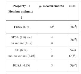
Table 6.1: A summary of the Hessian estimates presented in this chapter, along with their bias bounds.
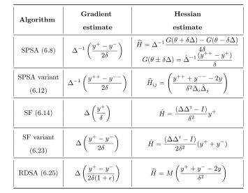
Table 6.2: A summary of the function measurements used and the form of gradient/Hessian estimates for the stochastic Newton algorithm (6.1). In the table, \(y^{++}\), \(y^{--}\), \(y^+\), \(y^-\), \(y\) denote the function measurements corresponding to input parameters \(\theta + \delta \Delta + \delta \hat \Delta\), \(\theta + \delta \Delta -\delta \hat \Delta\), \(\theta + \delta \Delta\), \(\theta - \delta \Delta\), and \(\theta\), respectively. The choice of random perturbation varies between rows. The matrix \(M\) used in the Hessian estimate presented in last row is defined in (6.27).
6.7 Asymptotic convergence of stochastic Newton algorithms
We consider the following coupled sequence of updates for the analysis of the Hessian recursion:
\[ \begin{align*} \theta_{n+1} &= \Gamma\left(\theta_n - a(n) \Theta\left( \overline{H}_n\right)^{-1} \widehat\nabla f(\theta_n)\right), \tag{6.34} \\ \overline{H}_{n+1} &=\overline{H}_n + b(n)(\hat{H}_n - \overline{H}_n), \tag{6.35} \end{align*} \]
where the quantity \(\hat{H}_n\) in (6.35) can correspond to any of the simultaneous perturbation Hessian estimators described in Chapter 6. Also, \(\widehat\nabla f(\theta_n)\) could be any of the simultaneous perturbation gradient estimators described in Chapter 3. As can be seen, it makes better sense from a computational perspective to have a similar class of estimators for both gradient and Hessian estimation. Thus, for instance, if one incorporates two-measurement SF for gradient estimation, the same two measurements can then also be used as in (6.23) for estimating the objective function Hessian. We consider here the case of a diminishing \(\{\delta_n\}\), i.e., \(0<\delta_n\rightarrow 0\) as \(n\rightarrow\infty\).
In (6.34), \(\Gamma:\mathbb{R}^d\rightarrow C\subset \mathbb{R}^d\) is a projection operator, where \(C\) is a compact and convex set. Also, in the above, \(\Theta:\mathbb{R}^{d\times d}\rightarrow \mbox{ } \{\mbox{positive definite }\) and symmetric \(d\times d\mbox{ matrices}\}\) is a projection operator that projects any \(d\times d\) matrix to the space of positive definite and symmetric matrices. Such an operator is needed to ensure that the algorithm proceeds in a descent direction. If a matrix \(A\) is already positive definite and symmetric, then \(\Theta\) is chosen such that \(\Theta(A)=A\) itself.
The operator \(\Theta\) can be characterized using methods such as the modified Choleski factorization procedure, see (D. P. Bertsekas 1999), or the procedures in (J. C. Spall 2000) as well as (X. Zhu and Spall 2002). For a matrix \(A\), let \((\Theta(A))^{-1}\) denote the inverse of \(\Theta(A)\) which is also positive definite and symmetric.
Assumption A6.8.
For any two sequences of \(d\times d\) matrices \(\{A_n\}\) and \(\{B_n\}\), \({\displaystyle \lim_{n\rightarrow \infty} \norm{\Theta(A_n)- \Theta(B_n)}=0}\) if \({\displaystyle \lim_{n\rightarrow \infty} \norm{A_n-B_n} = 0}\).
We have
\[ \sup_n \|\Theta(C_n)\| <\infty, \mbox{ } \sup_n \|(\Theta(C_n))^{-1}\| <\infty, \]
if \({\displaystyle \sup_n \|C_n\| <\infty}\) for a given sequence \(\{C_n\}\) of \(d\times d\) matrices.
The requirement in Assumption A6.8(i) can be easily imposed, see (D. P. Bertsekas 1999; J. C. Spall 2000; X. Zhu and Spall 2002). Further, a sufficient condition for Assumption A6.8(ii) is
\[ c_1\| z\|^2 \leq z^T \Theta(C_n)z \leq c_2 \| z\|^2, \tag{6.36} \]
for all \(z\in \mathbb{R}^d\), \(n\geq 0\). Most projection operators are seen to satisfy (6.36), see (Bhatnagar 2005) for a detailed discussion.
Assumption A6.9.
The step size schedules \(\{a(n)\}\) and \(\{b(n)\}\) together with the perturbation sequence \(\{\delta_n\}\) of positive real numbers satisfy the following:
\[ \sum_n a(n) = \sum_n b(n) =\infty, \tag{6.37} \]
\[ \sum_n \left(\frac{a(n)}{\delta_n}\right)^2 < \infty; \mbox{ } \sum_n \left(\frac{b(n)}{\delta_n^2}\right)^2 <\infty, \tag{6.38} \]
\[ \lim_{n\rightarrow \infty} \left(\frac{a(n)}{b(n)}\right) = 0. \tag{6.39} \]
Note that (6.37) ensures that the algorithm does not exhibit premature convergence as trajectories obtained by putting the parameters in (6.34) and (6.35) along time points obtained from the sequences \(\{a(n)\}\) and \(\{b(n)\}\), respectively, and obtaining continuous linear interpolations of these. This helps in arguing that these continuously interpolated trajectories asymptotically track the limit points of corresponding ODEs provided the noise in the sample observations vanishes asymptotically. The latter happens from (6.38). The first condition in (6.38) is the same as the corresponding condition for gradient based schemes (see Chapter 4. The second condition is necessitated from the form of the Hessian estimators in Chapter 6 where \(\delta_n^2\) appears in the denominator of the Hessian estimator, see for instance, (6.23). As with gradient-based schemes, one can show convergence of the resulting martingale sequence obtained from the Hessian estimator under the second condition in (6.38). Finally, (6.39) results in a difference in timescales within the recursions (6.34)-(6.35). In particular, it ensures that the Hessian update (6.35) proceeds on a faster scale as compared to the \(\theta\)-recursion (6.34) that makes use of the inverse of the projected Hessian update.
Assumption A6.10.
The function \(f\) is four-times continuously differentiable with \(\left|\nabla^4_{i_1, i_2, i_3, i_4} f(\theta) \right| < \infty\), for \(i_1, i_2, i_3,i_4=1,\ldots, d\) and for all \(\theta\in \R^d\).
Assumption A6.10 is the same as Assumption A6.1 (restated here for ease of reference).
Assumption A6.11.
We have
\[ \left\| E\left[\left. \widehat \nabla f(\theta_n)\right |\theta_n \right] - \nabla f(\theta_n) \right\| = O(\delta_n^2), \]
where \(\widehat \nabla f(\theta_n)\) and \(\nabla f(\theta_n)\) are the gradient estimate and the true gradient respectively.
\[ \left\| E\left[\left. \widehat H_n\right |\theta_n \right] - \nabla^2 f(\theta_n) \right\| = O(\delta_n^2), \]
where \(\widehat H_n\) and \(\nabla^2f(\theta_n)\) are respectively the Hessian estimate and the true Hessian respectively.
Assumptions A6.11(i) and A6.11(ii) have been shown to hold for the various gradient and Hessian estimators based on random perturbations in Chapters 3 and 6 respectively.
Lemma 6.4.
The sequence of Hessian updates \(\{\overline{H}_{n}\}\) is uniformly bounded with probability one. In other words, \(\sup_n \|\overline{H}_n\| <\infty\) a.s.
Proof.
Note that (6.35) can be rewritten as
\[ \begin{align*} \overline{H}_{n+1} &= \overline{H}_n + b(n)(\nabla^2f(\theta_n) + \xi_n +M_{n+1} - \overline{H}_n), \tag{6.40} \\ &= \overline{H}_n + b(n) (\nabla^2f(\theta_n) + \xi_n-\overline{H}_n) + b(n)M_{n+1}, \tag{6.41} \end{align*} \]
where \({\displaystyle \xi_n =E[\hat{H}_n|\theta_n]-\nabla^2f(\theta_n)}\). From Assumption A6.11, \(\xi_n=O(\delta_n^2)\rightarrow 0\) as \(n\rightarrow\infty\). Let us ignore for a moment, the term \(b(n)M_{n+1}\) in (6.41). Then, from Assumption A6.10 and the fact that \(\theta_n\in C\) (a compact set), it follows that \(\sup_n\|\nabla^2f(\theta_n)\|<\infty\). It also follows from Assumption A6.9 that \(b(n)\rightarrow 0\) as \(n\rightarrow\infty\). Thus, outside a set of probability zero, \(\exists N_0\geq 1\) such that \(\overline{H}_{n+1}\) (upon ignoring the \(b(n)M_{n+1}\) term in (6.41)) can be viewed as a convex combination of \(\overline{H}_n\) and a uniformly bounded quantity. Finally, observe that \({\displaystyle M_{n+1}= \hat{H}_n - E[\hat{H}_n|\theta_n]}\) is a martingale difference term. It can now be argued as before, using the step-size condition (6.38), and the martingale convergence theorem for square-integrable martingales, see Theorem B.7, that \({\sum_{m} b(m) M_{m+1}<\infty}\) a.s. Thus, \(\{\overline{H}_n\}\) as in (6.41) is uniformly bounded almost surely. The claim follows.
\(\square\)
As described in Chapter 2.7, the system of ODEs corresponding to (6.34)-(6.35) when viewed from the faster timescale are the following:
\[ \begin{align*} \dot{\theta}(t) &= 0, \tag{6.42} \\ \dot{\overline{H}}(t) &= \nabla^2 f(\theta(t))-\overline{H}(t). \tag{6.43} \end{align*} \]
In the light of (6.42), as also discussed in Chapter 2.7, one may let \(\theta(t)\equiv \theta\), \(\forall t\). Thus, (6.43) can then be rewritten as
\[ \dot{\overline{H}}(t) = \nabla^2 f(\theta)-\overline{H}(t). \tag{6.44} \]
The ODE (6.44) has \(\overline{H}^*(\theta) =\nabla^2 f(\theta)\) as its unique globally asymptotically stable attractor. By Assumption A6.10 and the fact that \(\theta\in C\), a compact set, \(\overline{H}^*(\theta)\) is Lipschitz continuous in \(\theta\).
Lemma 6.5.
We have
\[ \lim_{n\rightarrow\infty} \norm{\overline{H}_n - \overline{H}^*(\theta_n)} = 0, \mbox{ a.s.} \]
Proof.
An application of Theorem 2.2 on (6.35) gives us
\[ \|\overline{H}_n - E[\hat{H}_n|\theta_n]\| \rightarrow 0 \mbox{ a.s.,} \]
as \(n\rightarrow\infty\). The claim follows from an application of the triangle inequality and Assumption A6.11.
\(\square\)
Lemma 6.6.
We have
\[ \norm{\Theta(\overline{H}_n)^{-1} - \Theta(\overline{H}^*(\theta_n))^{-1}} = \norm{\Theta(\overline{H}_n)^{-1} - \Theta(\nabla^2 f(\theta_n))^{-1}} \rightarrow 0, \]
as \(n\rightarrow\infty\), a.s.
Proof.
The equality in the claim follows because \(\overline{H}^*(\theta_n) = \nabla^2 f(\theta_n)\). Now note that
\[ \begin{align*} &\norm{\Theta(\overline{H}_n)^{-1} - \Theta(\nabla^2 f(\theta_n))^{-1}} \\ &=\norm{\Theta(\nabla^2 f(\theta_n))^{-1} \left( \Theta(\nabla^2 f(\theta_n))\Theta(\overline{H}_n)^{-1} - I\right)} \\ &= \norm{\Theta(\nabla^2 f(\theta_n))^{-1} \left( \Theta(\nabla^2 f(\theta_n))\Theta(\overline{H}_n)^{-1} - \Theta(\overline{H}_n)\Theta(\overline{H}_n)^{-1}\right) } \\ &= \norm{\Theta(\nabla^2 f(\theta_n))^{-1} \left( \Theta(\nabla^2 f(\theta_n)) - \Theta(\overline{H}_n)\right) \Theta(\overline{H}_n)^{-1}} \\ &\leq \norm{\Theta(\nabla^2 f(\theta_n))^{-1}} \norm{ \Theta(\nabla^2 f(\theta_n)) - \Theta(\overline{H}_n)} \norm{\Theta(\overline{H}_n)^{-1}} \\ &\leq \sup_n \norm{\Theta(\nabla^2 f(\theta_n))^{-1}} \sup_n \norm{\Theta(\overline{H}_n)^{-1}} \norm{\Theta(\nabla^2 f(\theta_n)) - \Theta(\overline{H}_n)} \\ &\longrightarrow 0 \mbox{ as } n\rightarrow\infty, \mbox{ a.s.} \end{align*} \]
The first inequality follows from the property on induced matrix norms, cf. Proposition A.12 of (D. Bertsekas and Tsitsiklis 1989). Note also the following: (i) From Assumption A6.10 and the fact that \(\theta\in C\) (a compact set), \(\sup_n \|\nabla^2 f(\theta_n)\|\leq \bar{K} <\infty\), for some \(\bar{K}>0\) and by Assumption A6.8(ii), \(\sup_n \|\Theta(\nabla^2 f(\theta_n))^{-1}\|<\infty\) a.s. (ii) By Lemma 6.4, \(\sup_n\|\overline{H}_n\|<\infty\) a.s. Thus, by Assumption A6.8(ii), \(\sup_n \|\Theta(\overline{H}_n)^{-1}\|<\infty\) a.s. (iii) Finally, \(\|\Theta(\overline{H}_n)-\Theta(\nabla^2 f(\theta_n))\|\rightarrow 0\) as \(n\rightarrow\infty\) from Assumption A6.8(i) and Lemma 6.5.
\(\square\)
We now shift our attention to the slower timescale recursion (6.34). Consider the following ODE associated with (6.34):
\[ \dot{\theta}(t) = - \bar{\Gamma}\left(\Theta(\nabla^2 f(\theta(t)))^{-1} \nabla f(\theta(t))\right). \tag{6.45} \]
Here, \(\bar{\Gamma}: {\cal C}(C)\rightarrow {\cal C}({\cal R}^d)\) is defined according to
\[ \bar{\Gamma}(v(x)) = \lim_{\eta\rightarrow 0} \left(\frac{\Gamma(x+\eta v(x))-x}{\eta}\right), \tag{6.46} \]
for any continuous \(v:C\rightarrow {\cal R}^d\).
Let \(A\subset H\stackrel{\triangle}{=} \{\theta\in \mathbb{R}^d| \nabla f(\theta)=0\}\) be the set of globally asymptotically stable attractors for the ODE (6.45). In fact, \(V(\cdot) = f(\cdot)\) serves as a Lyapunov function for this ODE since
\[ \frac{dV(\theta)}{dt} = \nabla V(\theta)^T \dot{\theta} \]
\[ = \nabla f(\theta)^T \bar{\Gamma}\left( -\Theta(\nabla^2 f(\theta(t)))^{-1} \nabla f(\theta(t))\right) \leq 0, \]
since \(\Theta(\nabla^2 f(\theta))^{-1}\) is a positive definite matrix for each \(\theta\).
Theorem 6.7.
The recursion (6.34) satisfies \(\theta_n\rightarrow A\) a.s., as \(n\rightarrow \infty\).
Proof.
As a consequence of Lemma 6.6, we have
\[ \begin{align*} \theta_{n+1}&=\Gamma\left(\theta_n - a(n) \Theta(\overline{H}_n)^{-1} \widehat\nabla f(\theta_n)\right) \\ &= \Gamma\left(\theta_n - a(n) (\Theta(\overline{H}^*(\theta_n))^{-1}\nabla f(\theta_n) - \kappa_n)\right) \\ &= \Gamma\left(\theta_n -a(n) (\Theta(\nabla^2 f(\theta_n))^{-1} \nabla f(\theta_n) - \kappa_n)\right), \end{align*} \]
where \({\displaystyle \kappa_n = \Theta(\nabla^2 f(\theta_n))^{-1} \nabla f(\theta_n) - \Theta(\overline{H}_n)^{-1}\widehat\nabla f(\theta_n)}\). Now note that we can rewrite \(\kappa_n\) as
\[ \begin{align*} \kappa_n &= \Theta(\nabla^2 f(\theta_n))^{-1} (\nabla f(\theta_n) -\widehat\nabla f(\theta_n)) \\ &\qquad + (\Theta(\nabla^2 f(\theta_n))^{-1} - \Theta(\overline{H}_n)^{-1})\widehat\nabla f(\theta_n) \\ &= \Theta(\nabla^2 f(\theta_n))^{-1} (\nabla f(\theta_n) -\widehat\nabla f(\theta_n)) \\ &\qquad + (\Theta(\nabla^2 f(\theta_n))^{-1} - \Theta(\overline{H}_n)^{-1})\nabla f(\theta_n) \\ & \qquad+ (\Theta(\nabla^2 f(\theta_n))^{-1} - \Theta(\overline{H}_n)^{-1})(\widehat\nabla f(\theta_n) -\nabla f(\theta_n)). \end{align*} \]
Thus,
\[ \begin{align*} \norm{\kappa_n} &\leq \norm{\Theta(\nabla^2 f(\theta_n))^{-1}} \norm{\nabla f(\theta_n) -\widehat\nabla f(\theta_n)} \\ &\quad + \norm{\Theta(\nabla^2 f(\theta_n))^{-1} - \Theta(\overline{H}_n)^{-1}} \norm{\nabla f(\theta_n)} \\ &\quad + \norm{\Theta(\nabla^2 f(\theta_n))^{-1} - \Theta(\overline{H}_n)^{-1}} \norm{\widehat\nabla f(\theta_n) -\nabla f(\theta_n)}. \end{align*} \]
From Assumption A6.11(i), \(\norm{ \widehat\nabla f(\theta_n) -\nabla f(\theta_n)} = O(\delta_n^2)\rightarrow 0\) as \(n\rightarrow\infty\) and from Lemma 6.6, \(\norm{\Theta(\nabla^2 f(\theta_n))^{-1} - \Theta(\overline{H}_n)^{-1}} \rightarrow 0\) as \(n\rightarrow\infty\). Thus, \(\norm{\Theta(\nabla^2 f(\theta_n))^{-1} - \Theta(\overline{H}_n)^{-1}} \norm{\widehat\nabla f(\theta_n) -\nabla f(\theta_n)}\rightarrow 0\) as \(n\rightarrow\infty\). Further, from Assumption A6.10 and the fact that \(\theta_n\in C\), \(\forall n\), \(\sup_n \norm{\nabla f(\theta_n)} \leq \check{M}<\infty\) for some \(\check{M}>0\). Likewise from Assumption A6.10 together with the fact that \(\theta_n\in C\) (a compact set) and Assumption A6.8(ii), it follows that \(\sup_n \norm{\Theta(\nabla^2 f(\theta_n))^{-1}} \leq \check{N} <\infty\), for some \(\check{N}>0\). Thus, \(\norm{\kappa_n} \rightarrow 0\) as \(n\rightarrow\infty\) a.s.
Now observe that \(\nabla f(\theta)\) is continuous in \(\theta\) (by Assumption A6.10). Further, \(\nabla^2f(\theta)\) is continuous in \(\theta\) by Assumption A6.10 and \(\Theta(\nabla^2f(\theta))\) is also continuous by Assumption A6.8. It can also be shown as in Lemma 6.6 that \(\Theta(\nabla^2 f(\theta))^{-1}\) is continuous. Thus, the function \(F(\theta) = \Theta(\nabla^2 f(\theta))^{-1} \nabla f(\theta)\) is continuous. Thus, Assumption A2.9 holds. Now, from Assumption A6.9, it follows that \({\displaystyle \sum_n a(n)=\infty}\), \(a(n)\rightarrow 0\) as \(n\rightarrow\infty\), thereby satisfying Assumption A2.10. Further, using the identification \(\beta_n=\kappa_n\) with \(\norm{\kappa_n}\rightarrow 0\) a.s. as \(n\rightarrow\infty\), Assumption A2.11 can be seen to be satisfied. Finally, Assumption A2.12 is trivially satisfied since \(\eta_n=0\), \(\forall n\) (in our case). The claim now follows from Theorem 2.5 (the Kushner-Clark theorem for projected stochastic approximation, cf. Chapter 5 of (Kushner and Clark 1978)).
\(\square\)
6.8 Bibliographic remarks
Hessian estimation
In (Fabian 1971), the author analyzes a finite differences Hessian estimation scheme with \(O(d^2)\) function measurements. In an importance advance, the author in (J. C. Spall 2000) brings the idea of simultaneous perturbation for Hessian estimation, using random perturbations similar to those employed in SPSA. The advantage with this scheme is the drastic reduction in the number of function measurements to four, irrespective of the dimension. Subsequent advances that we presented in Sections 6.3.2, 6.5 are based on (Bhatnagar and Prashanth 2015) and (Prashanth et al. 2017), respectively.
Gaussian smoothed functional — an idea explored in Chapter 3 for estimating gradients, can be extended to estimate the Hessian as well. In Section 6.4.1 and 6.4.2, we presented two Gaussian SF schemes for Hessian estimation, and these are adapted from (Bhatnagar 2007). Proposition 6.1 is extracted from the proof of the bias of 1SF estimation in (Bhatnagar 2007), and this result has also been separately shown in later works, cf. (Erdogdu 2016; Balasubramanian and Ghadimi 2022). These works provide the connection of the result in Proposition 6.1 to the classic Stein’s identity, which includes a first as well as second-order variant, see (Stein 1972, 1981) and also (Balasubramanian and Ghadimi 2022 Theorem 1.2). Proposition 6.1 is central to the analysis of SF1 as well as SF2 estimators, in particular, to provide bounds of \(O(\delta)\) and \(O(\delta^2)\) on the bias of these estimators, respectively.
Zeroth-order Stochastic Newton
There is considerable work on Newton-based algorithms though not as much as for gradient-based schemes. In some early work, the Hessian is estimated using finite difference approximations that are in turn finite difference estimates of the gradients (Fabian 1971). Such a scheme however requires \(O(d^2)\) samples of the objective function at each update epoch. In (Ruppert 1985), it is assumed that the objective function gradients are known and these are in turn used to estimate the Hessian at each update instant. Zeroth-order simultaneous perturbation Hessian estimates have been developed for the first time in (J. C. Spall 2000) and Newton-based algorithms studied. The Hessian estimator here requires four function measurements. A procedure for projecting the Hessian to the space of positive definite and symmetric matrices is proposed. In (X. Zhu and Spall 2002), another method for projecting the eigenvalues to the positive half line is proposed for the algorithm in (J. C. Spall 2000). Certain feedback and weighting mechanisms for obtaining improved Hessian estimates have been proposed in (James C. Spall 2009).
Building on the work in (J. C. Spall 2000), four Newton algorithms have been developed and studied in (Bhatnagar 2005) that require four, three, two and one simulations, respectively, for estimating the Hessian regardless of the parameter dimension \(d\). In (Bhatnagar 2007), two smoothed functional algorithms based on Gaussian perturbations have been presented that require one and two function measurements, respectively. In (Bhatnagar and Prashanth 2015), a balanced SPSA based Hessian estimator is presented that requires three function measurements. Efficient ways of obtaining the Hessian inverse – a direct method and another procedure based on the Sherman-Morrison-Woodbury identity are also proposed here. The latter technique has also been made use of to obtain an efficient procedure in (Rastogi, Zhu, and Spall 2016). In (Ghoshdastidar, Dukkipati, and Bhatnagar 2014), a family of Newton algorithms based on q-Gaussian perturbations is presented. Here, one gets a wide range of smoothing functionals depending on the value of \(q\) with Gaussian, Cauchy and Uniform emerging as special cases for different values of the \(q\) parameter.
In (James C. Spall 2009), the sequence \(\{b(n\}\) is optimized for asymptotic variance of the Hessian estimator in terms of the perturbation sensitivity parameters \(\delta_n,n\geq 0\). We do not consider here this variance optimization problem in terms of the step-sizes \(b(n),n\geq 0\). In (J. Zhu, Wang, and Spall 2019), an efficient method for reducing the number of floating point operations from \(O(d^3)\) to \(O(d^2)\) is presented that is based on the symmetric indefinite matrix factorization approach presented in (Bunch and Parlett 1971). The method seems highly effective and stable, especially in high-dimensional problems.
Here \(\nabla^4 f(\theta) = \dfrac{\partial^4 f (\theta)}{\partial \theta\tr \partial \theta\tr \partial \theta\tr \partial \theta\tr}\) denotes the fourth derivative of \(f\) at \(\theta\) and \(\nabla^4_{i_1, i_2, i_3, i_4} f(\theta)\) denotes the \((i_1, i_2, i_3, i_4)\)th entry of \(\nabla^4 f(\theta)\), for \(i_1, i_2, i_3,i_4=1,\ldots, d\).↩︎