Appendix A — ODEs and differential inclusions
In this appendix, we review some of the key concepts from ordinary differential equations and differential inclusions. This background material is useful for the asymptotic analysis of stochastic approximation algorithms and stochastic recursive inclusions.
A.1 Ordinary differential equations
We consider the following ODE, that is the same as (2.2). We shall describe limit sets and notions of stability for such an ODE.
\[ \dot{\theta}(t) = h(\theta(t)). \tag{A.1} \]
We recall first the Gronwall inequality, a fundamental result useful for showing stability properties of ODEs, see Lemma B.1 of (Borkar 2022), for a proof.
Lemma A.1 (Gronwall Inequality).
Suppose that for continuous \(u,v:[0,T] \rightarrow [0,\infty)\), for \(T>0\) and scalars \(C,K\geq 0\):
\[ u(t) \leq C + K\int_{0}^{t} u(s)v(s) ds, \mbox{ }\forall t\in [0,T]. \]
Then it follows that for all \(t\in [0,T]\),
\[ u(t) \leq C \exp\left(K\int_{0}^{T} v(s)ds\right). \]
A.1.1 Limit sets of ODE
We present first some basic definitions on the limit sets of ODEs. Consider the ODE (A.1) with the function \(h:\mathbb{R}^d\rightarrow\mathbb{R}^d\) being Lipschitz continuous. In other words, \(\exists L>0\) (a constant) such that
\[ \|h(\eta)-h(\beta)\| \leq L\|\eta-\beta\|, \mbox{ } \forall \eta,\beta\in\mathbb{R}^d. \]
Definition A.1.
We say that the ODE (A.1) is well-posed if for any initial condition \(\theta_0\in\mathbb{R}^d\), there is a unique solution \(\theta(\cdot) \in C([0,\infty); \mathbb{R}^d)\) that is also continuous as a function of \(\theta_0\).
In the above, \(C([0,\infty);\mathbb{R}^d)\) denotes the space of all continuous functions from \([0,\infty)\) to \(\mathbb{R}^d\). The integral solution to the ODE (A.1) is obtained as
\[ \theta(t) = \theta_0 + \int_{0}^{t} h(\theta(s))ds, \mbox{ } t\geq 0. \tag{A.2} \]
If an ODE is well-posed, it has unique integral curves. The following theorem says that a sufficient condition for well-posedness of (A.1) is that the function \(h\) be Lipschitz continuous, see Theorem B.1 of (Borkar 2022) for a proof based on the Gronwall inequality (Lemma A.1).
Theorem A.2.
Suppose the function \(h:\mathbb{R}^d\rightarrow\mathbb{R}^d\) is Lipschitz continuous. Then the ODE (A.1) is well-posed.
For the ODE (A.1), let \(\Phi: \mathbb{R}\times \mathbb{R}^d\rightarrow \mathbb{R}^d\) be defined as the map \(\Phi(t,x)\stackrel{\triangle}{=} \Phi_t(x)\) that takes \(\theta(0)\) to \(\theta(t)\) via the ODE (A.1). Thus,
\[ \theta(t)=\Phi_t(\theta(0)) = \theta(0) +\int_{\tau=0}^{t} h(\Phi_\tau(\theta(0)))d\tau. \]
Assuming \(h\) is Lipschitz continuous, it follows from Theorem A.2 that the map \(\Phi\) is continuous. It is easy to verify that \(\{\Phi_t, t\in \mathbb{R}\}\) forms a group since \(\Phi_t \circ \Phi_s = \Phi_{t+s}\), \(\forall t,s\in \mathbb{R}\) and \(\Phi_0 =I\) (the identity map). Thus, \(\{\Phi_t,t\in \mathbb{R}\}\) is a flow of \(h\), see (Benaïm 1996), for a more general discussion.
Definition A.2 (Invariant sets and Periodic Points).
We say that \(A\subset \mathbb{R}^d\) is invariant for the ODE (A.1) if \(\Phi_t(A) \subset A\) for all \(t\in\mathbb{R}\).
We say that \(A\subset \mathbb{R}^d\) is positively (resp. negatively) invariant for the ODE (A.1) if \(\Phi_t(A) \subset A\) for all \(t\geq 0\) (resp. \(t\leq 0\)).
A point \(\theta\) is a periodic point for the ODE (A.1) if \(\exists T>0\) such that \(\Phi_T(\theta)=\theta\).
Note that since the flow \(\Phi\) is induced by the vector field \(h\), equilibria of (A.1) coincide with the zeros of the function \(h(\cdot)\). Further, both periodic points and equilibria can be viewed as recurrent points.
Definition A.3 (Limit Sets of an ODE).
Given a trajectory \(\theta(\cdot)\) of (A.1) with \(\theta(0)=\theta_0\in \mathbb{R}^d\), the orbit through \(\theta_0\) is the set
\[ \mathcal{O}(\theta_0) = \{ \theta(t) \in \mathbb{R}^d |t\in \mathbb{R}\}. \]
Given a trajectory \(\theta(\cdot)\) of (A.1), the set \(\mathcal{L} \stackrel{\triangle}{=} \cap_{t\geq 0} \overline{\theta([t,\infty))}\) that comprises of the set of limit points of (A.1) is called the \(\omega\)-limit set of (A.1).
Given \(\delta,T>0\), a \((\delta,T)\)-pseudo-orbit from \(\lambda\in \mathbb{R}^d\) to \(\eta\in\mathbb{R}^d\) is defined as a set of \(k\) trajectories of (A.1) (for some \(k<\infty\)): \(\{\Phi_t(\eta_i): t\in[0,t_i]\), \(t_i\geq T\}\), \(i=0,1,\ldots,k-1\), where \(\eta_0,\eta_1,\ldots,\eta_k\in \mathbb{R}^d\) and such that (i) \(\|\eta_0-\lambda\|<\delta\), (ii) \(\|\Phi_{t_j}(\eta_j) - \eta_{j+1}\| <\delta\), \(\forall j=0,1,\ldots,k-1\), and (iii) \(\eta_k=\eta\).
If a \((\delta,T)\)-pseudo-orbit exists between any \(\lambda,\eta\in \mathbb{R}^d\), for every \(\delta,T>0\), we say that the flow \(\Phi\) of (A.1) is chain transitive.
The flow \(\Phi\) as above restricted to \(\eta=\lambda\), for all \(\lambda\in\mathbb{R}^d\) is called chain recurrent.
A compact invariant set \(A\subset \mathcal{R}^d\) on which the flow \(\Phi\) of the ODE (A.1) is chain recurrent (resp. chain transitive) is called an internally chain recurrent (resp. internally chain transitive) set for (A.1).
We now recall the following result, see (Benaïm 1999 Proposition 5.3):
Lemma A.3.
Let \(A\subset \mathcal{R}^d\) be a compact invariant set for the ODE (A.1). The following are equivalent:
\(A\) is internally chain transitive.
\(A\) is connected and internally chain recurrent.
Definition A.4 (Equilibria and Attractors of an ODE).
A point \(\theta\in\mathbb{R}^d\) is an equilibrium of the ODE (A.1) if \(\Phi_t(\theta)=\theta\), \(\forall t\). In other words, \(h(\theta)=0\).
An equilibrium \(\theta\in\mathbb{R}^d\) of (A.1) is said to be isolated, if there exists an open set \(U\subset \mathbb{R}^d\) such that \(\theta\in U\) and there does not exist any other equilibrium \(\check{\theta}\in U\).
A compact invariant set \(A\subset \mathbb{R}^d\) is said to be Lyapunov stable or simply stable for the ODE (A.1) if given any \(\epsilon>0\), \(\exists \delta>0\) such that \(d(\theta_0,A)<\delta\) implies that \(d(\Phi_t(\theta(0)),A)<\epsilon\) for all \(t>0\). Here for any given \(x\in\mathbb{R}^d\), \(d(x,A) = \min_{\eta\in A} \|x-\eta\|\) is the distance between \(x\) and the set \(A\).
A set \(A\subset \mathbb{R}^d\) is an attractor for (A.1) if \(A\) is nonempty, compact and invariant. Further, \(A\) has a positively invariant open neighborhood \(M\subset \mathbb{R}^d\) such that \(d(\Phi_t(\theta), A) \rightarrow 0\) as \(t\rightarrow\infty\) uniformly in \(\theta\in M\).
The largest open neighborhood \(M\) for an attractor \(A\) above is called the domain of attraction of \(A\).
A compact invariant \(A \subset \mathbb{R}^d\) is asymptotically stable for the ODE (A.1) if it is both Lyapunov stable and an attractor.
We now mention the following important results in Lemmas A.4–A.6, see for instance, (Nandakumaran, Datti, and George 2017) for a detailed treatment.
Lemma A.4.
Suppose \(\theta(\cdot)\) is a solution of (A.1). Then \(\theta_l(t) = \theta(t+l)\) is also a solution to (A.1) for any fixed \(l\) and for all \(t\).
Lemma A.5.
Let \(\theta(\cdot)\) be a solution to the ODE (A.1) and \({\displaystyle \lim_{t\rightarrow\infty} \theta(t) = \bar{\theta}}\) for some \(\bar{\theta}\in \mathbb{R}^d\). Then \(\bar{\theta}\) is an equilibrium of (A.1).
Proof.
From Lemma A.4, for any \(l>0\), \(\theta(t+l)\), \(t\geq 0\), is also a solution to (A.1) and \({\displaystyle \lim_{t\rightarrow\infty} \theta(t+l)=\bar{\theta}}\). By the mean value theorem,
\[ \theta(t+l)-\theta(t) = l \dot{\theta}(\bar{t}) = l h(\theta(\bar{t})), \]
for some \(\bar{t} \in [t, t+l]\). Thus, as \(t\rightarrow \infty\), \(\bar{t}\rightarrow\infty\) as well, and \(\theta(t+l)-\theta(t)\rightarrow 0\) as \(t\rightarrow\infty\). By continuity, this implies that \(lh(\bar{\theta})=0\), hence \(h(\bar{\theta})=0\).
\(\square\)
Linearized System
Consider the ODE (A.1) and assume that the function \(h:\mathbb{R}^d\rightarrow\mathbb{R}^d\) is twice continuously differentiable. Let \(\bar{\theta}\in\mathbb{R}^d\) be an equilibrium of (A.1). Then by a Taylor’s expansion, we get
\[ h(\bar{\theta}+\theta) = h(\bar{\theta}) + Dh(\bar{\theta})\theta + O(\|\theta\|^2), \]
where
\[ Dh(\bar{\theta}) = \left[ \begin{array}{cccc} \nabla_1 h_1(\bar{\theta}) & \nabla_1 h_2(\bar{\theta})& \cdots& \nabla_1 h_d(\bar{\theta})\\ \nabla_2 h_1(\bar{\theta}) & \nabla_2 h_2(\bar{\theta})& \cdots& \nabla_2 h_d(\bar{\theta})\\ \cdots & \cdots &\cdots &\cdots\\ \nabla_d h_1(\bar{\theta}) & \nabla_d h_2(\bar{\theta})& \cdots & \nabla_d h_d(\bar{\theta})\\ \end{array} \right] \]
is the Jacobian of the function \(h=(h_1,h_2,\ldots,h_d)\) evaluated at \(\bar{\theta}\). Now note that \(h(\bar{\theta})=0\). If we ignore the higher order terms \(O(\|\theta\|^2)\), we get the linearized ODE:
\[ \dot{\theta}(t) = Dh(\bar{\theta}) \theta(t). \]
Lemma A.6.
If all the eigenvalues of \(Dh(\bar{\theta})\) have negative real parts, then \(\bar{\theta}\) is asymptotically stable for the ODE (A.1).
Sufficient Condition for Asymptotic Stability
Before proceeding further, we give a sufficient condition for verifying asymptotic stability of an attractor \(A\subset \mathbb{R}^d\) of the ODE (A.1). Let \(V:M\subset \mathbb{R}^d\rightarrow \mathbb{R}\) be a non-negative, continuously differentiable function. Suppose it satisfies the following condition:
\[ \langle \nabla V(\theta), h(\theta)\rangle \left\{ \begin{array}{ll} & <0 \mbox{ if }\theta \in M\cap A^c \\ & =0 \mbox{ if } \theta \in A. \end{array}\right. \]
The function \(h(\cdot)\) above is the driving vector field of the ODE (A.1). The asymptotic stability of \(A\) follows since \({\displaystyle \frac{d}{dt} V(\theta(t) \leq 0}\) with equality only for \(\theta(t) \in A\).
We now recall the Lasalle Invariance Principle, see Theorem 2 of (Lasalle and Lefschetz 1961).
Gradient Systems
Suppose the underlying system is a gradient scheme with the corresponding ODE being
\[ \dot{\theta}(t) = -\nabla f(\theta(t)), \mbox{ } \theta(0) =\theta_0. \tag{A.3} \]
Thus, here \(h(\theta)=-\nabla f(\theta)\). Note that
\[ \begin{align*} \frac{df(\theta(t))}{dt} &= - \nabla f(\theta(t))^T\nabla f(\theta(t)) \\ &= -\|\nabla f(\theta(t))\|^2 \\ & <0& \mbox{ if } \nabla f(\theta) \not= 0 \\ & =0& \mbox{ otherwise.} \end{align*} \]
Assuming \(f\geq 0\), the function \(f\) itself serves as a Lyapunov function with the set \(H=\{\theta|\nabla f(\theta)=0\}\) as the set of equilibrium points of (A.3). If \(f\) is not non-negative but bounded below, i.e., \(\exists C<0\) such that \(\min_x f(x)=C\). Then, one may let \(V(x)=f(x)+|C|\), which will ensure that \(V\geq 0\) and the above continues to hold.
We recall now Lemma 11.1 of (Borkar 2022).
Lemma A.8.
The only invariant sets that can occur as \(w\)-limit sets for the ODE (A.3) are the subsets of \(H\stackrel{\triangle}{=} \{\theta\in\mathbb{R}^d|\nabla f(\theta)=0\}\).
Lasalle Invariance Principle, see Theorem A.7, in the case of gradient systems, would say something similar as below.
Lemma A.9.
Any trajectory \(\theta(\cdot)\) of the ODE (A.3) with \(f\) as above must converge to the largest invariant set contained in \(H \stackrel{\triangle}{=}\{\theta\mid \nabla f(\theta)=0\}\).
A.2 Set-valued maps and differential inclusions
In many real life situations, one often encounters problems that are ill-posed, the solution is not unique, or there are uncertainties and imprecise modeling errors. Such problems arise often in stochastic control and optimization, reinforcement learning, viability theory and stochastic games. In such scenarios, one may not encounter single-valued maps at all and more general analytical techniques are needed. In this section, we present a brief background on set-valued maps and differential inclusions for which we refer primarily to the books (Aubin and Frankowska 1990) and (Aubin and Cellina 1984).
A.2.1 Set-valued maps
A set-valued map \(x\mapsto h(x)\) is one where for any \(x\in \mathbb{R}^n\), \(h:\mathbb{R}^n \rightarrow \{\)subsets of \(\mathbb{R}^m\}\) and is specified via it’s graph, i.e., Graph\((J) = \{(x,y)\mid y\in h(x)\}\). The domain (Dom\((h)\)) and image (Im\((h)\)) are respectively given by \({\displaystyle \mbox{Dom}(h) =\{x\in \mathbb{R}^n\mid h(x)\not= \phi\}}\) and \({\displaystyle \mbox{Im}(h) = \cup_{x\in \mathbb{R}^n} h(x)}\), respectively. The inverse \(h^{-1}\) of the set-valued map \(h\) (above) is also a set-valued map such that \(x\in h^{-1}(y)\) if and only if \(y\in h(x)\), viz., \((x,y) \in \mbox{Graph}(h)\).
The open ball of radius \(\epsilon\) around the origin is denoted \(B_\epsilon(0)\), while the closed ball is denoted \(\overline{B}_\epsilon(0)\). Thus, \(B_\epsilon(0) = \{x\in \mathbb{R}^n \mid \lVert x \rVert < \epsilon\}\) and \(\overline{B}_\epsilon(0) = \{x\in\mathbb{R}^n \mid \lVert x \rVert \le \epsilon\}\). For any set \(A\subset \mathbb{R}^n\), for any \(\delta >0\), we call \(N_\delta(A) = \{x\in\mathbb{R}^n\mid \|x-y\|<\delta, y\in A\}\) the \(\delta\)-open neighborhood or simply the neighborhood of the set \(A\). The \(\delta\)-closed neighborhood of \(A\) is likewise the set \(\overline{N^\delta}(A) = \{x\mid \|x-y\| \leq \delta, y\in A\}\).
We now have the following definitions pertaining to set-valued maps. Let \(h:\mathbb{R}^n \rightarrow \{\)subsets of \(\mathbb{R}^m\}\) be a set-valued map.
Definition A.5 (Continuity of Set-Valued Maps).
\(h\) is said to be upper semi-continuous at a point \(x\in \mbox{Dom}(J)\) if given sequences \(\{ x_{k} \}_{k \ge 1}\) (in \(\mathbb{R}^{n}\)) and \(\{ y_{k} \}_{k \ge 1}\) (in \(\mathbb{R}^{m}\)) with \(x_{k} \to x\), \(y_{k} \to y\) and \(y_{k} \in h(x_k)\), \(\forall k \ge 1\), we have \(y \in h(x)\). We say that \(h\) is upper semi-continuous if it is upper semi-continuous at every \(x\in \mbox{Dom}(h)\). In other words, Graph\((h)\) is closed.
\(h\) is said to be lower semi-continuous at a point \(x\in \mbox{Dom}(h)\) if for any \(y\in h(x)\), and any sequence of points \(x_k \in \mbox{Dom}(h)\) converging to \(x\), there exists a sequence of elements \(y_k \in h(x_k) \to y\in h(x)\). We say that \(h\) is lower semi-continuous if it is lower semi-continuous at every \(x\in \mbox{Dom}(h)\).
\(h\) is continuous at \(x\in \mbox{Dom}(h)\) if it is both upper semi-continuous and lower semi-continuous at \(x\). It is said to be continuous if and only if it is continuous at every \(x\in \mbox{Dom}(h)\).
\(h\) is Lipschitz at \(z\in \mathbb{R}^n\) if there exists \(L>0\) and \(\epsilon>0\) such that for all \(x,y\in N_\epsilon(\{z\})\), we have that \(h(x) \subset h(y) + L\|x-y\|B_1(0)\) where \(B_1(0)=\{w\in\mathbb{R}^m\mid \|w\|<1\}\) is a unit ball around the origin in \(\mathbb{R}^m\) or more compactly \(h(x) \subset N_{L\|x-y\|}(h(y))\).
It is important to note here that there exist set-valued maps that are upper semi-continuous but not lower semi-continuous and vice versa.
Definition A.6 (Peano or Marchaud Map).
A set-valued map \(h:\mathbb{R}^n \rightarrow \{\)subsets of \(\mathbb{R}^m\}\) is called a Peano or Marchaud map if it satisfies the following properties:
For every \(x\in\mathbb{R}^n\), \(h(x)\) is convex and compact.
\(h\) is pointwise bounded for every \(x\in\mathbb{R}^n\), i.e., for some \(K>0\) we have, \({\displaystyle \sup_{w\in h(x)} \|w\| \leq K(1+\|x\|)}\).
\(h\) is upper semi-continuous, see Definition A.5(i).
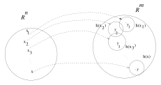
Figure A.1: A set-valued map \(h:\mathbb{R}^n\rightarrow \{\mbox{subsets of }\mathbb{R}^m\}\) is called a Peano or marchaud map if (i) \(h(x)\) is compact and convex for every \(x\), (ii) \(h(x)\) is pointwise bounded and (iii) \(h\) is upper semi-continuous.
The distance of a point \(x\in \mathbb{R}^d\) to a set \(A\subset \mathbb{R}^d\) (for any \(d\geq 1\)) is defined as \(d(x,A)=\inf\{\|x-y\| \mid y\in A\}\). Notice that a point \(x_0\in\mathbb{R}^d\) is a boundary point of \(A\) if and only if \(d(x,A)=d(x,A^c)=0\).
Definition A.7 (Limsup and Liminf of Set-Valued Maps).
Given a set-valued map \(h:\mathbb{R}^n\rightarrow \{\mbox{subsets of } \mathbb{R}^m\}\), we define the upper limit (Limsup) and lower limit (Liminf) of the sequence of sets \(h(x_k)\) as follows:
Limsup\(_{x_k\rightarrow x} h(x_k) = \{y\in\mathbb{R}^m\mid \liminf_{x_k\rightarrow x}d(y,h(x_k))=0\}\).
Liminf\(_{x_k\rightarrow x} h(x_k) = \{y\in\mathbb{R}^m\mid \lim_{x_k\rightarrow x}d(y,h(x_k))=0\}\).
Note that both Liminf and Limsup are closed sets. Liminf collects the limit points of \(\{h(x_k)\}\) while Limsup collects its accumulation points. Further, \(\mbox{Liminf}_{x_k\rightarrow x}h(x_k) \subset \overline{h(x)} \subset \mbox{Limsup}_{x_k\rightarrow x} h(x_k)\).
A.2.2 Differential inclusions
A differential inclusion (DI) can be viewed as a generalization of an ODE in the sense that it involves set-valued maps as opposed to the usual point-to-point maps and in general has the form
\[ \dot{x}(t) \in h(t,x(t)), \tag{A.4} \]
where \(h:\mathbb{R}\times \mathbb{R}^d \rightarrow \{\mbox{subsets of }\mathbb{R}^d\}\). We shall mainly be interested with the case where \(h(t,x)\stackrel{\triangle}{=}h(x)\), i.e., there is no explicit time dependence of the set-valued map \(h\). In such a case, \(h(x)\subset \mathbb{R}^d\), for any \(x\in \mathbb{R}^d\). Thus, the DI in this case takes the form
\[ \dot{x}(t) \in h(x(t)), \tag{A.5} \]
with \(h:\mathbb{R}^d \rightarrow \{\mbox{subsets of }\mathbb{R}^d\}\). Any solution to (A.5) is viewed in the Caratheodory sense, i.e., as an absolutely continuous function satisfying (A.5) almost everywhere.
Definition A.8.
Let \(K\subset \mbox{Dom}(h)\). A function \(x:[0,T]\rightarrow \mathbb{R}^d\) is said to be viable in \(K\) if \(x(t) \in K\), \(\forall t\in [0,T]\).
A solution \(x(\cdot)\) to (A.5) is said to be viable if for some closed subset \(K\) of Dom\((h)\), we have that \(x(t)\in K\), \(\forall t\).
For \(K\subset \mathbb{R}^d\), given \(x\in \bar{K}\) (the closure of \(K\)), the contingent cone is defined by
\[ C(x,K) \stackrel{\triangle}{=} \left\{y\in \mathbb{R}^d\mid \liminf_{k\rightarrow 0^+} \frac{d(x+ky,K)}{k}=0\right\}. \]
We say that a set \(K\subset \mbox{Dom}(h)\) is a viability domain of the set-valued map \(h\) if and only if for all \(x\in K\), \(h(x) \cap C(x,K) \not= \phi\).
Consider the case where \(K= \{{x}\}\). Then the contingent cone to \(\{{x}\}\) is given by \(C(x,\{x\}) = \left\{y\mid \liminf_{k\rightarrow 0^+} \frac{d(x+ky, \{x\})}{k} =0\right\} = \{0\}\). Then, from Definition A.8(iv), it follows that \(K=\{x\}\) is a viability domain of \(h\) if and only if \(h(x) \cap \{0\} \not=\phi\) or \(x\) is a stationary solution to the inclusion \(0\in h(x)\) implying that \(x\) is an equilibrium of \(h\). Thus, the minimal viability domains are equilibria of set-valued maps. We now recall the following results from (Aubin and Frankowska 1990) (see Theorems 10.1.12-10.1.13 there).
Theorem A.10.
Consider a Peano or Marchaud map \(h:\mathbb{R}^d \rightarrow \{\)subsets of \(\mathbb{R}^d\}\). Then the limit sets of the solutions to the DI (A.5) are closed viability domains. Further, the limit of a solution \(x(t)\) to the DI (A.5) (if it exists), as \(t\rightarrow\infty\), is an equilibrium of \(h\).
Theorem A.11.
Let \(h:\mathbb{R}^d \rightarrow \{\)subsets of \(\mathbb{R}^d\}\) be a Peano or Marchaud map. If \(K\subset \mbox{Dom}(h)\) is a compact viability domain and if \(h(K)\) is convex, then there exists an equilibrium of \(h\) in \(K\).
A.2.3 Limit Sets of Differential Inclusions
Recall that a solution to the DI (A.5) is an absolutely continuous mapping \(\mathbf{x}:\mathbb{R}\rightarrow \mathbb{R}^d\) such that \(\mathbf{x}(0)=x\) and \(\dot{\mathbf{x}}(t) \in h(\mathbf{x}(t))\) for almost every \(t\in\mathbb{R}\). The \(\omega\)-limit set of a given solution \(\mathbf{x}\) of the DI (A.5) with \(\mathbf{x}(0) = x\) is given by \(L({x}) = \bigcap_{t \ge 0} \ \overline{\mathbf{x}([t, +\infty))}\).
Consider \(\{\Phi_t\}_{t\in\mathbb{R}}\) defined by \(\Phi_t(x) = \{\textbf{x}(t) \ | \ \textbf{x}\) is a solution to the DI (A.5) with \(\textbf{x}(0) = x \}\). Then \(\{\Phi_t\}\) is the set-valued semi-flow associated with the DI (A.5). For \(B \times M \subset \mathbb{R} \times \mathbb{R}^d\), we let \({\displaystyle \Phi_B(M) = {\bigcup}_{t\in B, x\in M} \Phi_t (x)}\). For \(M\subset \mathbb{R}^d\), the \(\omega\)-limit set for the DI (A.5) is specified by (cf. (Benaïm, Hofbauer, and Sorin 2005)) \({\displaystyle \omega_\Phi(M) = \bigcap_{t\geq 0} \overline{\Phi_{[t,+\infty)}(M)}}\).
Definition A.9 (Invariance of Sets).
Let \(M \subset \mathbb{R}^d\). We say that
\(M\) is strongly invariant if \(M=\Phi_t(M)\) for every \(t \in \mathbb{R}\).
\(M\) is quasi-invariant if \(M \subset \Phi_t(M)\), \(\forall t\in\mathbb{R}\).
\(M\) is semi-invariant if \(\Phi_t(M)\subset M\), \(\forall t\in\mathbb{R}\).
\(M\) is strongly positively invariant if \(\Phi_t(M) \subset M\), \(\forall t>0\).
\(M\) is invariant (for the set-valued map \(h\)) if \(\forall x\in M\), \(\exists\) a solution \(\mathbf{x}\) to the DI (A.5) with \(\mathbf{x}(0)=x_0\) and with \(\mathbf{x}(\mathbb{R}) \subset M\).
Definition A.10 (\((\epsilon,T)\)-Chain).
Given a set \(M\subset \mathbb{R}^d\), and \(x,y\in M\), by an \((\epsilon, T)\)-chain from \(x\) to \(y\), we mean a sequence \(\{\mathbf{x}_1,\ldots,\mathbf{x}_n\}\), for some integer \(n\geq 1\), of solutions to the DI (A.5) together with real numbers \(t_1,\ldots,t_n>T\), such that
\(\mathbf{x}_i(s) \in M\), \(\forall 0\leq s\leq t_i\) and \(i=1,\ldots,n\),
\(\|\mathbf{x}_i(t_i) - \mathbf{x}_{i+1}(0)\| \leq \epsilon\), for all \(i=1,\ldots,n-1\),
\(\|\mathbf{x}_1(0)-x\| \leq \epsilon\) and \(\|\mathbf{x}_n(t_n)-y\|\leq\epsilon\).
Definition A.11 (Internally Chain Transitive and Chain Recurrent Sets).
We define these sets as follows:
The set \(M\subset\mathbb{R}^d\) is said to be internally chain transitive for the DI (A.5) if \(M\) is compact and for any \(x,y\in M\), there exists an \((\epsilon,T)\)-chain for any \(\epsilon,T>0\).
If the property in part (i) above holds only for all \(x=y\in M\), then the set \(M\) is said to be chain recurrent.
Definition A.12 (Perturbed Solution to a DI).
A function \(z:[0,\infty)\rightarrow \mathbb{R}^d\) is said to be a perturbed solution to (A.5) if the following hold:
\(z\) is absolutely continuous.
There exists a locally integrable function \(U:[0,\infty)\rightarrow \mathbb{R}^d\) such that
\({\displaystyle \lim_{t\rightarrow\infty} \sup_{0\leq v\leq T} \| \int_{t}^{t+v} U(s)ds \|=0}\) for all \(T>0\).
\({\displaystyle \frac{dy(t)}{dt} - U(t) \in h^{\delta(t)}(y(t))}\) for almost every \(t>0\), for some \(\delta:[0,\infty)\rightarrow\mathbb{R}\) such that \(\delta(t)\rightarrow 0\) as \(t\rightarrow\infty\). Here \(h^\delta(y) = \{x\in \mathbb{R}^d\mid \exists z\) s.t. \(\|z-x\| <\delta, d(x,h(z)) <\delta\}\).
We now state a couple of important results, see (Benaïm, Hofbauer, and Sorin 2005 Lemma 3.5 and Theorem 3.6).
Lemma A.12.
Any internally chain transitive set for the DI (A.5) is invariant.
Theorem A.13.
Let \(\mathbf{z}\) be a bounded perturbed solution to the DI (A.5) with \(\mathbf{z}(0)=z\). Then the limit set of \(\mathbf{z}\) given by \({\displaystyle L({z}) = \bigcap_{t\geq 0} \overline{\{\mathbf{z}[t,+\infty)\}}}\) is internally chain transitive for (A.5).
Definition A.13 (Attracting/Attractor and Lyapunov Stable Sets for a DI).
In relation to the DI (A.5), we have the following definitions:
\(A \subseteq \mathbb{R}^d\) is said to be an attracting set if it is compact and there exists a neighborhood \(U\) such that for any \(\epsilon > 0\), \(\exists \ T(\epsilon) \ge 0\) with \(\Phi_{[T(\epsilon), +\infty)}(U) \subset N^{\epsilon}(A)\). In other words, any DI trajectory initiated in U reaches the \(\epsilon\)-neighborhood of \(A\), \(T(\epsilon)\) instants later and stays there forever subsequently.
The set \(U\) above is called the fundamental neighborhood of \(A\).
An attracting set \(A\) that is also invariant is called an attractor set.
The basin of attraction of \(A\) is the set \(B(A) = \{x\in\mathbb{R}^d \mid w_\Phi(x) \subset A\}\). In other words, this is the largest subset of \(\mathbb{R}^d\) such that the DI initiated anywhere within this set has its \(\omega\)-limit set contained in \(A\).
The set \(A\) is said to be Lyapunov stable if for all \(\delta > 0\), \(\exists \ \epsilon > 0\) such that \(\Phi_{[0, +\infty)}(N^\epsilon(A)) \subseteq N^\delta(A)\).
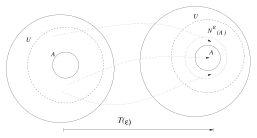
Figure A.2: The set \(A\) is attracting if (a) it is compact and (b) there is a neighborhood \(U\) of \(A\) such that given any \(\epsilon>0\), there exists \(T(\epsilon)>0\) so that any trajectory of the DI (A.5) starting in \(U\) arrives and stays within an \(\epsilon\)-neighborhood of \(A\) beyond an amount of time \(T(\epsilon)\) and subsequently stays in that neighborhood. Thus, \(\Phi_t(U) \in N^\epsilon(A)\), \(\forall t\in [T(\epsilon),\infty)\). The set \(A\) is an attractor if in addition it is also invariant.
A.3 Bibliographic Remarks
Differential equations have been well studied over many centuries with starting work primarily in the areas of physical and mechanical systems. Both Isaac Newton and Gottfried Leibniz are credited to have done early work in differential equations in the late 17th century. Early textbook treatments of ODEs include (Ince 1956; Coddington, Levinson, and Teichmann 1956). Excellent, more recent, texts include (Arnold 1992; Hirsch, Smale, and Devaney 2013; Nandakumaran, Datti, and George 2017). An excellent treatment on differential equations with discontinuous right hand sides is given in (Filippov 2013). Applications of such equations in many engineering domains have been well studied, for instance, see (Andronov, Vitt, and Khaikin 2013) for a recent English translation of a Russian text of the 1950’s by these authors. Differential inclusions is a more general framework for dynamical systems that have differential equations with non-unique solutions resulting from lack of Lipschitz continuity and possibly even discontinuity of the right hand sides. Excellent texts on differential inclusions include (Aubin and Frankowska 1990; Aubin and Cellina 1984). We finally remark that a set-valued map \(h\) as in Definition A.6 has been referred to as Peano map in (Aubin and Frankowska 1990) and as Marchaud map in (Benaïm, Hofbauer, and Sorin 2005).
A.4 Exercises
Exercise 1.
A function \(V(\theta)\) satisfying \(V(0)=0\) and \(V(\theta)>0\) for \(\theta\ne 0\) is said to be positive-definite. For \(V(\theta) = a \theta_1^2+2\theta_1 \theta_3+a \theta_2^2+4 \theta_2 \theta_3+a \theta_3^2\), identify the range of \(a\) that ensures positive-definiteness of \(V\).
Exercise 2.
Consider the ODE \(\dot \theta(t)= A \theta(t),\) where \(A=\begin{bmatrix} 0 & -1\\1 & -1 \end{bmatrix}\). Answer the following:
Is this system asymptotically stable?
Suppose \(V(\theta)=\theta\tr P \theta\) for some matrix symmetric, positive-definite \(P\) that ensures \(P A + A\tr P\) is negative-definite. Show that \(V\) is a Lyapunov function for the linear system given above.
Exhibit a Lyapunov function for the system given above through an appropriate choice of \(P\).
Exercise 3.
Consider the ODE (A.1) with a Lipschitz continuous function \(h:\mathbb{R}^d\rightarrow\mathbb{R}^d\) with Lipschitz constant \(L>0\). Assume the ODE evolves over the time interval \([0,T]\) for some \(T>0\).
Writing the integral form (A.2) of the ODE with two different initial conditions \(\theta_1,\theta_2\in \mathbb{R}^d\), obtain trajectories \(\theta_1(t)\) and \(\theta_2(t), t\in [0,T]\), respectively.
Write down an inequality (upper bound) for \(\|\theta_1(t)-\theta_2(t)\|\), \(t\in [0,T]\), using Lipschitz continuity of the function \(h\).
Apply Gronwall’s inequality (cf. Lemma A.1) on the inequality above using the functions \(u,v:[0,T]\rightarrow [0,\infty)\), where \(u(t)=\|\theta_1(t)-\theta_2(t)\|\) and \(v(t)=1\), \(\forall t\in [0,T]\), to show that \(u(t)\) is Lipschitz continuous as a function of the initial condition \(u(0)\).
Exercise 4.
Find the equilibria of the ODE system
\[ \dot{\theta_1}= \theta_2, \mbox{ } \dot{\theta_2} = - K \sin(\theta_1), \]
for some \(K>0\). Are these equilibria isolated?
Exercise 5.
Consider the following ODE:
\[ \dot{\theta}(t) = A\theta(t) + b, \]
where \(A\) is a \(d\times d\) negative definite matrix, \(b\in \mathbb{R}^d\) is a given vector and \(\theta(t)\in \mathbb{R}^d, \forall t\geq 0\).
Identify equilibria for this ODE?
Does this ODE have any attractors? If so, identify them?
Show that the following serves as a Lyapunov function for the above ODE:
\[ W(\theta) = \frac{1}{2} (A\theta+b)^T (A\theta+b). \]
Exercise 6.
Consider the following ODE in \({\cal R}^d\):
\[ \dot{\theta}(t) = -P(\nabla^2 J(\theta(t)))^{-1} \nabla J(\theta(t)), \hspace{8pt} \theta(0) \in {\cal R}^d. \]
Here, \(J:{\cal R}^d \rightarrow R\) is a twice continuously differentiable function. Further, \(P\) is an operator that uniquely maps all symmetric matrices to the space of positive definite and symmetric matrices. Let \(\theta(t)\), \(t\geq 0\) denote a trajectory of the above ODE. Giving precise arguments, describe the behaviour of \(\theta(t)\) as \(t\rightarrow\infty\)? List down any assumptions that you may make.
Exercise 7.
Consider the following set-valued map:
\[ F(x) = \left\{ \begin{array}{ll} x & \mbox{ if } x<0\\ 1 & \mbox{ if } x>0. \end{array} \right. \]
Further, for \(x=0\), \(F(x)=[0,1]\). Giving precise arguments, show whether or not
\(F\) is a Peano or Marchaud map?
F is lower semicontinuous?
\(\{0\}\) is strongly positively invariant for \(F\)?
\(\{0\}\) is invariant for \(F\)?
Exercise 8.
Let \(F\) be the set-valued map on \(\mathbb{R}\) given by \(F(x) = -sgn(x)\) for \(x\not= 0\) and \(F(0)=[-1,1]\). Here \(sgn(x) = +1\) if \(x>0\) and equals \(-1\) otherwise.
Show that \(\{0\}\) is strongly positively invariant as well as invariant for the differential inclusion \(\dot{x}(t) \in F(x(t))\)?
Identify \(\Phi_t(0)\), show whether or not \(\{0\}\) is an attractor for the inclusion \(\dot{x}(t) \in F(x(t))\) and if so, also identify the attracting set?
Show that \(F(\cdot)\) is a Peano or Marchaud map?