7 Escaping saddle points
In Chapters 4 and 6, we provided theoretical guarantees that establish asymptotic convergence to a stationary point of the objective function \(f\). On the other hand, in Chapter 5, we established convergence of zeroth-order stochastic gradient algorithms to an approximate stationary point in the non-asymptotic regime. However, these results are not sufficient in a non-convex optimization setting since local maxima and saddle points are also stationary points in addition to local minima. We shall refer to such undesirable stationary points collectively as saddle points, as in the recent literature (Jin et al. 2017, 2021; R. Ge et al. 2015).
It is desirable to escape saddle points and converge to a local minimum. In several ML applications, it may be enough to avoid saddle points and converge to local minima, as such points may be as good as global minima in many applications. A few concrete applications that possess such a characteristic are as follows: low rank matrix factorization (Jin et al. 2017), tensor decomposition (R. Ge et al. 2015), matrix sensing (Bhojanapalli, Neyshabur, and Srebro 2016), dictionary learning (Sun, Qu, and Wright 2016), matrix completion (Rong Ge, Lee, and Ma 2016), robust principal component analysis (Rong Ge, Jin, and Zheng 2017), and a sub-class of neural networks (Kawaguchi 2016). In each of these applications, local minima are as good as global minima, while there are innumerable first-order stationary points that are not local minima. Moreover, at each such saddle point, there is a direction of escape corresponding to a negative eigenvalue.
We discuss two schemes to escape saddle points. This goal is also referred to as avoidance of traps, cf. (Borkar 2003; Barakat et al. 2021; Gadat and Gavra 2022). The first scheme is the vanilla ZSG algorithm presented earlier. We show that, when the noise in the function measurements is rich, then the ZSG algorithm, which employs the unified gradient estimate, converges to a local minimum asymptotically. We shall use the ODE approach for this result. The second scheme is a variant of the stochastic Newton algorithm, and incorporates a cubic-regularization term. We establish the convergence of the cubic-regularized Newton algorithm to an approximate second-order stationary point (SOSP) in the non-asymptotic regime. An SOSP would be a local minimum when the objective satisfies a strict saddle condition, made precise later.
The rest of this chapter is organized as follows: In Section 7.1, we introduce first and second-order stationary points. In Section 7.2, we present an asymptotic result for escaping saddle points for ZSG algorithm under assumptions on the measurement noise. In Section 7.3, we discuss two algorithms for escaping saddle points in a setting where exact gradient and Hessian measurements are available. The first algorithm uses curvature information, while the second one adds extraneous noise so that the iterates do not get stuck at a saddle point. In Section 7.4, we present the cubic-regularized Newton algorithm with zeroth-order gradient/Hessian estimates and provide a non-asymptotic sample complexity bound for identifying approximate SOSPs.
7.1 First and second-order stationary points
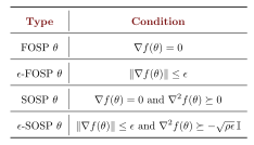
The non-asymptotic bounds in Chapter 5 were shown to converge to an approximate stationary point. Recall that, at a first-order stationary point (FOSP), say \(\bar \theta\), the gradient vanishes, i.e., \(\nabla f(\bar\theta)=0\). An \(\epsilon\)-approximation to FOSP is a point \(\bar\theta\) that satisfies \(\norm{\nabla f(\bar\theta)} \le \epsilon\).
Finding an FOSP is not sufficient for a non-convex objective function \(f\), as such a point is not necessarily a local minimum. As a simple example, consider \(f(\theta_1,\theta_2)=\theta_1^2 - \theta_2^2\). Then, \(\nabla f(0,0)=0\), implying \((0,0)\) is an FOSP. However, the origin is clearly not a local minimum because \(f(0,\epsilon) < f(0,0)\) for any \(\epsilon\).
As illustrated in Figure 7.1, an FOSP could potentially be a saddle point. In order to avoid such points and find local optima of \(f\), we need information with regard to the curvature of the underlying objective. The notion of second-order stationary point (SOSP) formalizes this idea and aids in escaping saddle points.
At a second-order stationary point (SOSP), say \(\bar\theta\), we have \(\nabla f(\bar\theta)=0\) and \(\lambda_{\min} \left( \nabla^2 f(\bar\theta) \right) \ge 0\), where as before, \(\lambda_{\min}(A)\) denotes the smallest eigenvalue of the \(d\times d\)-matrix \(A\).
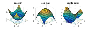
Figure 7.1: Illustration of three types of first-order stationary points. The image is sourced from offconvex.org
For the non-asymptotic analysis, an \(\epsilon\)-version of SOSP is defined below.
Definition 7.1 (\(\epsilon\)-second-order stationary point).
Fix \(\epsilon>0\). Let \(\theta_R\) be the output of a stochastic iterative algorithm for solving (1.1). Then, \(\theta_R\) is said to be an \(\epsilon\)-SOSP in expectation if
\[ \begin{align*} \max \left\{ \sqrt{\E{\norm{\nabla f(\theta_R)}}}, \frac{-1}{\sqrt{\rho}} \E{\lambda_{\min} \left( \nabla^2 f(\theta_R) \right) } \right\} \!\le \!\sqrt{\epsilon}, \tag{7.1} \end{align*} \]
where \(\rho\) is a positive parameter.
From the definition above, in expectation, \(\theta_R\) can be inferred to be a point where the size (or norm) of the objective gradient is small, and the Hessian at \(\theta_R\) is nearly positive semi-definite. Thus, \(\theta_R\) is an approximation to a point where the objective gradient vanishes and the Hessian is positive semi-definite. We next elaborate on the subtleties behind finding such a point.
If \(\nabla f(\theta)=0\) and \(\nabla^2 f(\theta) \succ 0\), then one can conclude that \(\theta\) is a local minimum. On the other hand, if \(\nabla f(\theta)=0\) and \(\nabla^2 f(\theta) \succeq 0\), then one has to go beyond a SOSP and look at the third derivatives to infer if \(\theta\) is a local minimum or not, and so on. Such a process is not amenable for optimization using gradient-based methods, as there is no end to calculating higher-order derivatives with the hope of finding a local minimum. Staying within the realm of first and second derivatives (or the gradient and Hessian), we would like to understand conditions that guarantee that a candidate point is a local minimum and not a saddle point. At an FOSP, if the Hessian is positive definite (resp. negative definite), we have a local minimum (resp. local maximum). If the Hessian is indefinite, i.e., has both positive and negative eigenvalues, then we have arrived at a saddle point and the negative eigenvalues can be used to move away from such a point. On the other hand, if the Hessian is degenerate, i.e., either positive or negative semi-definite, then the optimization process becomes hard, in particular, to find local minima. More precisely, it is well-known that finding a local minimum is an NP-hard problem, see (Anandkumar and Ge 2016). However, if the saddle points are strict, i.e., Hessian is not degenerate, then there exist polynomial time algorithms for finding a local minimum. The strict saddle condition is as follows:
\[ \begin{align*} \nabla f(\theta)=0\textrm{ and }\lambda_{\min}(\nabla^2 f(\theta)) < 0. \tag{7.2} \end{align*} \]
When the strict saddle condition (7.2) holds, an SOSP will be a local minimum since at a saddle point one can find a direction corresponding to a negative eigenvalue where the function decreases, whereas at an SOSP no such directions exist.
When the strict saddle condition (7.2) is satisfied, the Hessian \(\nabla^2 f(\theta)\) has at least one negative eigenvalue and this gives a direction for a method using second-order information to escape from saddle points. The cubic-regularized Newton algorithm presented in Section 7.4 uses the Hessian estimates to escape from a saddle point, and find an \(\epsilon\)-SOSP, as formalized in Definition 7.1, while using \(O\left(\frac{1}{\epsilon^{3.5}}\right)\) samples.
The table below summarizes the conditions for FOSP, SOSP and their approximate variants.
We conclude this section with a simple example, where SOSPs coincide with global minima.
Example 7.1 (Matrix factorization).
For a given positive semi-definite matrix \(M\), consider the following objective function:
\[ \begin{align*} \min_{\theta\in \R^d} \left\{f(\theta) = \frac{1}{2}\| \theta \theta\tr - M \|_F^2\right\}. \tag{7.3} \end{align*} \]
Let \(M = U \Lambda U\tr\), where \(\Lambda\) is a diagonal matrix with eigenvalues \(\lambda_1, \lambda_2, \dots, \lambda_d\), and the matrix \(U\) contains the eigenvectors of \(M\). Assume \(\lambda_1 > \lambda_2 \geq \dots \geq \lambda_d \geq 0.\) Let \(u_1, u_2, \dots, u_d\) denote the eigenvectors of \(M\) corresponding to the eigenvalues \(\lambda_1,\ldots,\lambda_d\).
The gradient and Hessian of \(f\) are given by
\[ \begin{align*} \nabla f(\theta) &= \|\theta\|_2^2 \theta - M\theta, \textrm{ and } \tag{7.4} \\ \nabla^2 f(\theta) &= \|\theta\|_2^2 I + 2\theta \theta\tr - M. \tag{7.5} \end{align*} \]
From the Hessian expression, it is apparent that the function \(f(\theta)\) is non-convex. Setting \(\nabla f(\theta)=0\), we obtain \(( \|\theta\|_2^2 I - M ) \theta = 0\) or \(M \theta=\|\theta\|_2^2 \theta\). Thus, the stationary points are zero and \(\pm \sqrt{\lambda_i} u_i\), for \(i=1,\ldots,d\).
For \(\theta = \sqrt{\lambda_i} u_i\), notice that \(f(\theta) = -\lambda_i^2 + \|M\|_F^2.\) Thus, \(f\) is minimized at \(\pm \sqrt{\lambda_1} u_1\). Moreover, using the expression of the Hessian above, a straightforward calculation shows that \(\nabla^2 f(\theta) \succeq 0\) at \(\pm \sqrt{\lambda_1} u_1\) and not at \(\pm \sqrt{\lambda_i} u_i\) for \(i\ne 1\). For the remaining local minima, say \(\tilde x\), since \(\lambda_1>\lambda_2\), we have a direction of escape using the top eigenvector \(u_1\), since \(u_1 \nabla^2 f(\tilde x)\tr u_1 \le \lambda_2-\lambda_1 <0\).
7.2 Asymptotic escaping of saddle points for ZSG algorithm
A common trick to escape saddle points is to add extraneous noise so that a stochastic gradient algorithm does not get stuck and instead, converges to a local minima. This approach is the adopted in (Jin et al. 2017, 2021; R. Ge et al. 2015). In particular, such a scheme, referred to as perturbed gradient descent, involves the following update iteration:
\[ \begin{align*} \theta_{n+1} = \theta_n - a(n) \left(\widehat \nabla f(\theta_n)+\zeta_n\right), \tag{7.6} \end{align*} \]
where \(\zeta_n\) is extraneous noise that is injected into the stochastic gradient algorithm, and is usually sampled from a zero-mean multivariate Gaussian vector with covariance matrix \(\sigma^2 I\). The extraneous noise ensures that the iterate \(\theta_n\), governed by (7.6), does not converge to an unstable equilibrium of the underlying ODE \(\dot \theta(t)= -\nabla f(\theta(t)),\) implying escape from saddle points. We shall explore this idea in more detail in the next section.
In this section, we adopt a different viewpoint, which is to show convergence to local minima for the case where the noise in the gradient estimates is rich in all directions, which in turn does not let the ZSG algorithm get stuck at an undesirable saddle point. Recall ZSG uses the following update:
\[ \begin{align*} \theta_{n+1} = \theta_n - a(n) \left(\widehat \nabla f(\theta_n)\right), \tag{7.7} \end{align*} \]
We shall use the unified gradient estimator described in Chapter 3. For the sake of readability, we recall this estimator below.
\[ \begin{align*} \widehat\nabla f(\theta_n) = \left(\frac{ y_n^+ - y_n^-}{2\delta}\right) V_n, \tag{7.8} \end{align*} \]
where \(y_n^+= f(\theta_n+\delta U_n)+\xi_n^+\), and \(y_n^- = f(\theta_n- \delta U_n)+\xi_n^-\). Notice that, unlike the asymptotic convergence analysis from Chapter 4, we employ a constant sensitivity parameter \(\delta>0\) and not a diminishing one. Such a choice aids the main result of this section, which establishes avoidance of saddle points for the update (7.7).
Under certain conditions on the measurement noise \(\{\xi_n^\pm\}\), one can avoid injecting noise artificially, and instead directly establish convergence to local minima, owing to the noise in the gradient estimator. The additional assumption on measurement noise is made precise below.
Assumption A7.1.
\(\exists\, c_3,c_4>0\) such that \(c_3\leq\E_k|\xi_k^+-\xi_k^-|\), where \(\E_k(\cdot)\) is shorthand notation for \(\E(\cdot\mid \F_k)\). In addition, \(|\xi_k^+-\xi_k^-| \leq c_4\), \(\forall k\).
The assumption above ensures that the noise in function measurements is rich in all directions.
Consider the following ODE:
\[ \begin{align*} \dot\theta(t)=- \E\left[\left.\left(\frac{ f(\theta(t)+\delta U) - f(\theta(t)-\delta U)}{2\delta}\right) V\right|\theta(t)\right], \tag{7.9} \end{align*} \]
where the expectation is over the joint distribution of \(U,V\).
Theorem 7.1.
Suppose the conditions of Proposition 3.1 and A7.1 hold. Further, assume \(\l V_k \r \le B_0\) a.s. for all \(k\). Set \(a(k) = \frac{c_5}{k^\alpha}\) and \(\delta_k=\delta,\, \forall k\), for some constants \(c_5, \delta>0\) and \(\alpha\in\left(\frac{1}{2},1\right]\). Then, \(\{\theta_k\}\) governed by (7.7), converges to the stable critical points of the ODE (7.9).
The result above says that the stochastic gradient algorithm (7.7) avoids unstable critical points of the ODE (7.9). However, the stable critical points of this ODE are not necessarily the local minima of the objective \(f\). A related ODE is \(\dot\theta(t)=-\nabla f(\theta(t)).\) By the bias bounds in Chapter 3, we know that
\[ \begin{align*} \left\|\E\left[\left.\left(\frac{ f(\theta+\delta U) - f(\theta-\delta U)}{2\delta}\right) V\right|\theta\right] - \nabla f(\theta)\right\| = O(\delta^2). \end{align*} \]
While the bias could in principle add spurious points (that are not local minima of \(f\)) to the limit set of (7.9), it is possible to find a \(\delta_0\) for any \(\epsilon>0\) such that for all \(\delta \le \delta_0\), the algorithm governed by (7.7) converges almost surely to an \(\epsilon\)-neighborhood of the local minima of \(f\), cf. Theorem 2.4 of (Bhatnagar et al. 2003).
For the proof, we require a result from (Pemantle 1990). We adapt this result to a gradient update and state it below.
Theorem 7.2 (Avoidance of traps).
Consider the following stochastic approximation update iteration:
\[ \begin{align*} \theta_{k+1} & = \theta_{k}+a(k) h(\theta_k) + \psi_k. \tag{7.10} \end{align*} \]
Suppose the following conditions hold.
\(\frac{c_5}{k^\alpha} \leq a(k) \leq \frac{c_6}{k^\alpha}\) for some constants \(c_5,c_6> 0\) and \(\alpha\in\bigg(\frac{1}{2},1\bigg]\);
\(\E_k\left[(\psi_k \cdot \vartheta)^+\right]\geq c_7/k^\alpha\) for some \(c_7> 0\) and every unit vector \(\vartheta\). Here \((a \cdot b)\) denotes the dot product between \(a\) and \(b\), and \((a)^+=\max(a,0)\);
\(\lVert \psi_k \rVert\leq c_8/k^\alpha\) for some \(c_8 > 0\).
Suppose \(h \in C^2\). Then, \(\{\theta_k\}\) governed by (7.10), converges to the stable critical points of the ODE \(\dot\theta(t)=h(\theta(t)).\)
We now prove Theorem 7.1.
Proof.
We first rewrite the update rule (7.7) as follows:
\[ \begin{align*} \theta_{k+1} &=\theta_{k}-a(k) \widehat \nabla f(\theta_k) \\ & = \theta_{k}-a(k)\nabla f(\theta_k) - \psi_k , \tag{7.11} \end{align*} \]
where \({\displaystyle \psi_k= a(k)\left[\frac{\xi_k^+-\xi^-_k}{\delta}V_k\right]}\).
The convergence of (7.11) to a local minimum can be inferred from Theorem 7.2 provided that conditions (B1)–(B3) of (Pemantle 1990) are satisfied.
It is easy to see that \(a(k)\) defined in the theorem statement satisfies condition (B1).
We now show that condition (B2) holds. Consider the unit vector \(\vartheta\) with the \(i\)th entry as \(1\). Letting \(V_k^i\) denote the \(i\)th entry of the vector \(V_k\), we have
\[ \begin{align*} &\E_{k}[(\psi_k\cdot\vartheta)^+]=\E_{k}\left[\frac{(a(k)(\xi_k^+-\xi_k^-) V_k^i)^+}{\delta} \right] \\ &\stackrel{(b)}{\ge}\E_{k}\left[\frac{a(k)(\xi_k^+-\xi_k^-) V_k^i+a(k)|(\xi_k^+-\xi_k^-)\, V_k^i|}{2\delta}\right] \\ &\stackrel{(c)}{=}\E_{k}\left[\frac{a(k)|\xi_k^+-\xi_k^-|\, |V_k^i|}{2\delta}\right] \\ &\stackrel{(d)}{\geq} \frac{c_5 c_3 \min\limits_{i=1\ldots,d}\E | V_k^i|}{2\delta k^\alpha}. \end{align*} \]
In the above, we used the fact that \(\max(x,y)=\frac{x+y+|x-y|}{2}\) to infer the equality in \((b)\). To infer the equality in \((c)\), we used \(\E_{{k}}[(\xi_k^+-\xi_k^-)V_k^i]=0\), which holds since \(\E_k[\xi_k^+-\xi_k^-]=0\) and \(V_k\) is independent of \(\mathcal{F}_k\). Finally, A7.1 allows us to infer \((d)\). Thus, condition (B2) holds.
We now turn to verifying condition (B3). Notice that
\[ \begin{align*} \lVert\psi_k\rVert &\le \frac{a(k)}{\delta}\lVert(\xi_k^+-\xi_k^-)V_k\rVert \le \frac{c_4 c_5 B_0}{\delta k^{\alpha}}, \end{align*} \]
where we used the following facts:
(a) \(\lVert(\xi_k^+-\xi_k^-)\rVert \le c_4\) from A7.1; (b) \(\lVert V_k\rVert\leq B_0\) by assumptions in the theorem statement; and (c) \(a(k) = \frac{c_5}{k^\alpha}\). Thus, condition (B3) holds.
The verification of conditions (B1)–(B3) above together with the fact \(f \in \C^3\) (by assumption) imply that (7.11) avoids unstable critical points of the ODE (7.9), by an invocation of Theorem 7.2.
\(\square\)
7.3 Escaping saddle points with exact gradient/Hessian measurements
In this section, we operate with exact gradient and/or Hessian measurements. We use this setting to illustrate the main algorithmic ideas to find an SOSP.
We make the following smoothness assumption for the sake of algorithmic development as well as analysis.
Assumption A7.2.
There exist positive scalars \(L_1, L_2\) such that
\[ \begin{align*} \norm{\nabla f(\theta_1) - \nabla f(\theta_2)} &\le L_1 \norm{\theta_1 - \theta_2}, \textrm{ and } \\ \norm{\nabla^2 f(\theta_1) - \nabla^2 f(\theta_2)} &\le L_2 \norm{\theta_1 - \theta_2}. \tag{7.12} \end{align*} \]
In addition, we shall assume a finite lower bound for the objective \(f\), made precise in the assumption below.
Assumption A7.3.
There exists a \(\bar f>-\infty\) s.t. \(f(\theta)\ge \bar f\) for all \(\theta \in \R^d\).
7.3.1 Hessian-aided scheme
Recall that, at an \(\epsilon\)-SOSP, we have \(\norm{\nabla f(\theta)}\le \epsilon\) and \(\lambda_{\min}(\nabla^2 f(\theta)) \ge -\sqrt{\epsilon}\). Finding a point with \(\norm{\nabla f(\theta)}\le \epsilon\) is easy and a simple GD algorithm would achieve this goal. This claim is made precise below for a GD update iteration given by
\[ \begin{align*} \theta_{k+1} = \theta_k - a \nabla f(\theta_k). \tag{7.13} \end{align*} \]
Since \(f\) is \(L_1\)-smooth and setting \(a < \frac{1}{L_1}\), we have
\[ \begin{align*} f(\theta_{k+1}) &\leq f(\theta_k) + \nabla f(\theta_k)\tr (\theta_{k+1}-\theta_k) + \frac{L_1}{2}\norm{\theta_{k+1}-\theta_k}^2 \\ &= f(\theta_k) - a \norm{\nabla f(\theta_k)}^2 + \frac{a^2L_1}{2}\norm{\nabla f(\theta_k)}^2 \\ & \leq f(\theta_k) - \frac{a}{2} \norm{\nabla f(\theta_k)}^2. \tag{7.14} \end{align*} \]
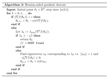
Thus, using the GD update (7.13), one could get to a point, say \(\bar \theta\), satisfying \(\norm{\nabla f(\bar\theta)}\le \epsilon\). However, such a point could be a saddle, and needs to be escaped from. A natural alternative is to use second-order information to move away from a potential saddle point. From an algorithmic viewpoint, one could perform a GD step (7.13) when the gradient is large, i.e., \(\norm{\nabla f(\theta)}> \epsilon\), and on arriving at a point with a small gradient, inspect the Hessian to infer if an SOSP is found. More precisely, let \(\lambda_k := \lambda_{\text{min}}(\nabla^2 f(\theta_k))\). If \(\lambda_k \ge -\sqrt{\epsilon}\), then an \(\epsilon\)-SOSP is found, since we inspect the Hessian \(\nabla^2 f(\theta_k)\) only if \(\norm{\nabla f(\theta)} \le \epsilon\). Otherwise, find an eigenvector, say \(u_k\), corresponding to \(\lambda_k\), with the additional constraint that \(\|u_k\| = 1\) and \(u_k\tr \nabla f(\theta_k) \leq 0\). Using this eigenvector, perform the following update iteration:
\[ \begin{align*} \theta_{k+1} = \theta_k + a(k) u_k. \tag{7.15} \end{align*} \]
Using Taylor expansions and the update given above, we obtain
\[ f(\theta_{k+1}) \leq f(\theta_k) + a(k) \nabla f(\theta_k)\tr u_k + \frac{1}{2} a(k)^2 u_k\tr \nabla^2 f(\theta_k) u_k + \frac{1}{6} L_2 a(k)^3 \|u_k\|^3. \]
Setting \(a(k)=\frac{2|\lambda_k|}{L_2}\), and using \(u_k\tr \nabla f(\theta_k) \leq 0\), we obtain
\[ \begin{align*} f(\theta_{k+1}) &\leq f(\theta_k) - \frac{1}{2} \frac{4\lambda_k^2}{L_2^2} |\lambda_k| + \frac{1}{6} L_2 \frac{8|\lambda_k|^3}{L_2^3}. \tag{7.16} \end{align*} \]
Thus, during each iteration of an algorithm that performs either (7.13) or (7.15), the function value drops. For a GD step (7.13), the decrease in function value is given by (7.14) and for the other step involving curvature information from the Hessian, the decrease in function value is given by (7.16). Now, the algorithm on termination, returns an SOSP. The termination in a finite number of iterations can be argued by the fact that the function value decreases in each iteration, and the maximum decrease is \(f(\theta_0)-f(\theta^*)\). Such a calculation would lead to an \(O(1/\epsilon^2)\) number of iterations for finding an \(\epsilon\)-SOSP.
Based on the discussion above, a two-step algorithm for finding SOSPs is given as a pseudocode in Algorithm 3.
The algorithm above has two drawbacks. First, it requires explicit Hessian computation. The cubic-regularized Newton algorithm in the next section overcomes this drawback by working with Hessian-vector products. The second drawback involves the computational overhead resulting from the update (7.15), which requires examining the eigenvalues of the Hessian. Even with Hessian vector products, the implementation is computationally expensive when compared to a GD update. We next discuss an alternative that is a variant of GD, which finds an SOSP.
7.3.2 Perturbed GD
Recall from the discussion in the section above that a GD step is appropriate when the gradient norm is large. On the other hand, when the gradient norm is small, then we have either found an SOSP or else a saddle point. To avoid the latter case, the algorithm from the section above inspected the Hessian, in particular, to infer if the minimum eigenvalue satisfies the SOSP condition or not. A computationally efficient alternative is to inject noise artificially when the latter condition holds, i.e., when gradient norm is small and the iterate has not moved much for many iterations. This idea forms the basis for perturbed GD1, with pseudocode in Algorithm 4.
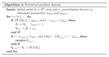
Algorithm 4 performs a regular GD step when the gradient is large, and as seen before, such a step would ensure a decrease in function value. However, when the gradient norm \(\norm{\nabla f(\theta_k)}\) is small, the algorithm may be either at a SOSP, or at a saddle point. To avoid the latter case, Algorithm 4 adds noise from an isotropic distribution. More precisely, as an intermediate step, when \(\norm{\nabla f(\theta_k)} \le g_{\text{thres}}\) for some threshold parameter \(g_{\text{thres}}\), and no noise has been added for a certain threshold \(t_{\text{thres}}\) number of iterations, Algorithm 4 would perturb the iterate as follows:
\[ \begin{align*} \theta_{k+1} = \theta_{k} + \zeta_k, \tag{7.17} \end{align*} \]
where \(\zeta_k\) is extraneous noise that could be chosen from an isotropic distribution. In essence, Algorithm 4 performs regular GD between two instants where the parameter is perturbed. The \(t_{\text{thres}}\) parameter ensures that these instants are separated in time well enough.
For a careful choice of parameters \(g_{\text{thres}}\), \(t_{\text{thres}}\), \(f_{\text{thres}}\) and the distribution of \(\zeta_k\), it can be shown that perturbed GD finds an \(\epsilon\)-SOSP in \(O(\log^4(d)/\epsilon^2)\) iterations. The result below makes this claim precise.
Theorem 7.4 (Theorem 3 of (Jin et al. 2017)).
Suppose Assumptions A7.2–A7.3 hold. Set perturbed GD algorithm’s parameters as follows: \(\chi =3\max\{\log\left(\frac{d\ell\Delta_f}{c\epsilon^2\delta}\right), 4\}, ~a = \frac{c}{\ell}, ~g_{\text{thres}} = \frac{\sqrt{c}}{\chi^2}\cdot \epsilon, ~f_{\text{thres}} = \frac{c}{\chi^3} \cdot \sqrt{\frac{\epsilon^3}{\rho}}, ~t_{\text{thres}} = \frac{\chi}{c^2}\cdot\frac{\ell}{\sqrt{\rho \epsilon}}\) \(t_{\text{noise}} = -t_{\text{thres}}-1\). Further, let the extraneous noise \(\zeta_k\) in Algorithm 4 be sampled uniformly from the surface of sphere with radius \(r = \frac{\sqrt{c}}{\chi^2}\cdot\frac{\epsilon}{\ell}\).
Then, there exists an absolute constant \(c_{\max}\) such that, for any \(\delta>0, \epsilon \le \frac{\ell^2}{\rho}\), \(\Delta_f \ge f(\theta_0) - f^\star\), and constant \(c \le c_{\max}\), perturbed GD will output an \(\epsilon\)-SOSP, with probability \(1-\delta\), and terminate in the following number of iterations:
\[ O\left(\frac{L_2(f(\theta_0) - f^\star)}{\epsilon^2}\log^{4}\left(\frac{dL_2\Delta_f}{\epsilon^2\delta}\right) \right). \]
Proof.
We provide a brief sketch of the main proof ideas below. We refer the reader to (Jin et al. 2017) for the complete proof.
Recall from the previous section that a GD step results in a function decrease given by
\[ \begin{align*} f(\theta_{k+1}) & \leq f(\theta_k) - \frac{a}{2} \norm{\nabla f(\theta_k)}^2. \tag{7.18} \end{align*} \]
Next, if \(\theta_k\) satisfies \(\norm{\nabla f(\theta_t)} \le g_{\text{thres}}\) and \(\lambda_{\min}(\nabla^2 f(\theta_k)) \le -\sqrt{\rho\epsilon}\), then adding one perturbation step (7.17) followed by \(t_{\text{thres}}\) GD steps, we have
\[ f(\theta_{k+t_{\text{thres}}}) - f(\theta_k) \le -f_{t_{\text{thres}}} \text{ with high probability}. \]
Thus, if Algorithm 4 is at a saddle point, then perturb and GD steps ensure a decrease in function value.
Next, at an SOSP, Algorithm 4 would either remain there, which is the favorable case, or move away, in which case there is a function value decrease.
Thus, there is a function value decrease with GD/perturbed GD steps, and the total number of iterations can be inferred using the average function value decrease per iteration. This calculation would be along similar lines as in the previous section for Algorithm 3 in the sense that the maximum decrease is \(f(\theta_0)-f^*\), and the algorithm either stops (with an SOSP), or continues to decrease the function value between iterations.
\(\square\)
We remark that Algorithm 4 has been extended to the case with stochastic gradients in (Jin et al. 2021). In particular, the aforementioned reference considers a setting where the gradient estimates are unbiased, and the noise in these estimates satisfy a certain sub-Gaussianity requirement. Under these conditions, the authors establish convergence of a variant Algorithm 4 with noisy gradient estimates to an approximate SOSP with high probability. However, to the best of our knowledge, a similar result is not available for Algorithm 4 in the zeroth-order setting, where the gradient estimates have a bias-variance tradeoff.
7.4 Cubic-regularized stochastic Newton
The standard Newton step is given by
\[ \theta_{k+1} = \theta_k - \nabla^2 f(\theta_k)^{-1} \nabla f(\theta_k). \]
This is equivalent to finding a \(\theta\) that minimizes a second-order approximation, i.e., the following:
\[ \begin{align*} &\theta_{k+1}= &\argmin_{\theta \in \mathbb{R}^d} \left\{ \!\innerproduct{\nabla f(\theta_k)}{\theta \! - \!\theta_k} \!+\! \frac{1}{2} \innerproduct{\nabla^2 f(\theta_k) (\theta \! - \!\theta_k)}{\theta \! - \!\theta_k} \right\}. \end{align*} \]
For the case of a convex objective, the Newton method finds minima efficiently as compared to a gradient method, since the former uses a second-order approximation. However, for a non-convex objective, the Newton method may not necessarily escape from saddle points. A fix is to have an incremental algorithm that performs either a gradient or a Newton step adaptively, with the decision for the type of the step based on the gradient norm at the current point. In particular, gradient steps for large gradients and Newton steps otherwise. Such a two-step algorithm, analyzed for deterministic optimization in (Wright and Recht 2022, sec. 3.6), finds an \(\epsilon\)-SOSP in \(O\left(\frac{1}{\epsilon^3}\right)\) number of iterations, where each iteration is either a gradient or Newton step. An elegant alternative to achieve the same effect as the two-step algorithm discussed above is cubic regularization, which is described next.
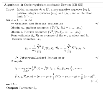
The cubic regularized Newton step adds a cubic term to the auxiliary function in the following manner:
\[ \begin{align*} \theta_{k+1} = \argmin_{\theta \in \mathbb{R}^d} &\bigg\{ \innerproduct{\nabla f(\theta_k)}{\theta - \theta_k} \\ &\quad+ \frac{1}{2} \innerproduct{\nabla^2 f(\theta_k) (\theta - \theta_k)}{\theta - \theta_k} + \frac{\alpha}{6} \norm{\theta - \theta_k}^3 \bigg\}, \end{align*} \]
where \(\alpha \in \mathbb{R}^{+}\) is the regularization parameter. Since the gradient and Hessian of \(f\) are not directly available, we obtain \(\widehat\nabla f(\theta_k,l), l=1,\ldots,m_k\) estimates of the gradient and \(\widehat\nabla^2 f(\theta_k,l), l=1,\ldots,b_k\) estimates of the Hessian at \(\theta_k\). We use an average of these estimates, denoted by \(\Bar g_k\) and \(\Bar \Hess_k\), respectively, to solve the cubic sub-problem (7.19) in each round of cubic-regularized stochastic Newton (CR-SN) algorithm, whose pseudocode is presented in Algorithm 5. The mean-squared error (MSE) of the gradient estimate \(\Bar g_k\) is \(O\left(\frac{1}{m_k}\right)\), whereas the corresponding bound for the Hessian estimate \(\Bar \Hess_k\) is \(O\left(\frac{1}{b_k}\right)\), see Lemma 7.7 below. We require the MSE to vanish asymptotically in order to ensure convergence of CR-SN to an \(\epsilon\)-SOSP of the objective.
We consider CR-SN under two different settings. In the first setting, the gradient and Hessian estimates are unbiased, whereas in the second setting, these estimates are biased. In the next section, we establish convergence of CR-SN to an approximate SOSP in the first setting, and subsequently, extend the analyses to cover the second setting.
7.4.1 The case of unbiased gradient/Hessian information
In this setting, the gradient/Hessian estimates satisfy the following assumption:
Assumption A7.4.
Let \(\F_k=\sigma(\theta_i, i\le k)\). Recall \(\E_k\) denotes the expectation conditioned on \(\F_k\). For any \(k \ge1\), we have
\(\E_k \left[ \widehat\nabla f(\theta_k)\right] = \nabla f \left(\theta_{k}\right) ,\) \(\E_k \left[ \widehat\nabla^2 f(\theta_k)\right] = \nabla^2 f \left(\theta_{k}\right)\).
\({ \E_k \left[ \left\| \widehat\nabla f(\theta_k) - \nabla f \left(\theta_{k}\right)\right\|^{2}\right] \leq \sigma_1^{2} },\)
\({ \E_k \left[ \left\| \widehat\nabla^2 f(\theta_k) - \nabla^2 f \left(\theta_{k}\right)\right\|^{2}\right] \leq \sigma_2^{2} }\), for some \(\sigma_1, \sigma_2 \ge 0\).
The assumption above is satisfied in a risk-neutral RL setting, for instance, see (Maniyar et al. 2024). On the other hand, in a risk-sensitive RL application, obtaining unbiased gradient/Hessian information is not feasible. Instead, one can use simultaneous perturbation-based gradient/Hessian estimators that are formed using function measurements. Such a setting involves biased gradient/Hessian estimates, which we shall analyze in the next section.
The result establishes convergence of Algorithm 5 to an \(\epsilon\)-SOSP.
Theorem 7.5.
Suppose Assumptions A7.4 and A7.2 hold. Let \(\{\theta_1, \dots, \theta_N\}\) be computed by Algorithm 5 with the following parameters:
\[ \begin{align*} \alpha_k &= 3 L_2, \quad N = \frac{12\sqrt{L_2} (f(\theta_0)-f^*)}{\epsilon^{\frac{3}{2}}}, \tag{7.20} \\ m_k &= \frac{25 \sigma_1^2}{4 \epsilon^2}, \quad b_k = \frac{36 \sqrt[3]{30 (1 + 2 \log 2d)} d^{\frac{2}{3}} \sigma_2^2}{L_2 \epsilon}. \tag{7.21} \end{align*} \]
Let \(\theta_R\) be picked uniformly at random from \(\{\theta_1, \ldots, \theta_N\}\). Then,
\[ \begin{align*} & 5 \sqrt{\epsilon} \ge \max \left\{ \sqrt{\E{\norm{\nabla f(\theta_R)}}}, \frac{-5}{6 \sqrt{L_2}} \E{\lambda_{\min} \left( \nabla^2 f(\theta_R) \right) } \right\}, \tag{7.22} \end{align*} \]
where \(L_1\) and \(L_2\) are specified in Assumption A7.2.
As we reduce the parameter \(\epsilon\), the batch sizes \(m_k,b_k\) as well as the number of iterations \(N\) can be seen to increase. Alternatively, the batch sizes increase with \(N\), and hence are not to be viewed as constants.
Proof of Theorem 7.5
The proof proceeds through a sequence of lemmas while following the technique from (Balasubramanian and Ghadimi 2022) and (Maniyar et al. 2024).
Lemma 7.6.
Let \(\Bar{\theta} = \argmin_{x \in \mathbb{R}^d} \Tilde{f}(x, \theta, \Hess, g, \alpha)\). Then, we have
\[ \begin{align*} &g + \Hess(\Bar{\theta}-\theta) + \frac{\alpha}{2}\norm{\Bar{\theta}-\theta}(\Bar{\theta}-\theta) = 0 , \tag{7.23} \\ &\Hess + \frac{\alpha}{2}\norm{\Bar{\theta}-\theta} I_d \succeq 0 . \tag{7.24} \end{align*} \]
where \(I_d\) is the identity matrix.
The result below provides error bounds for the gradient and Hessian estimates, which are sample averages.
Lemma 7.7.
Let \(\Bar{g}_k\) and \(\Bar{\Hess}_k\) be computed as in Algorithm 5, and assume \(m_k\ge 1\), \(b_k \ge 4(1 + 2\log 2d)\). Then,
\[ \begin{align*} \E{\norm{\Bar{g}_k - \nabla f(\theta_{k-1})}^2} &\le \frac{\sigma_1^2}{m_k} , \tag{7.25} \\ \E{ \norm{\Bar{\Hess}_k - \nabla^2 f(\theta_{k-1})}^3 } &\le \frac{4 \sqrt{15 (1 + 2\log 2d)} d \sigma_2^3}{ b_k^\frac{3}{2}}. \tag{7.26} \end{align*} \]
Proof.
Using Assumption A7.4, we have
\[ \begin{align*} & \E{\norm{\Bar{g}_k - \nabla f(\theta_{k-1})}^2} \\ &= \E{ \norm{ \frac{1}{m_k} \sum_{l=1}^{m_k} \left( \widehat\nabla f(\theta_{k-1},l) - \nabla f(\theta_{k-1})\right)}^2 } \le \frac{\sigma_1^2}{m_k}. \end{align*} \]
This establishes the first bound in (7.25). Now we turn to proving the second bound in (7.25). By Theorem 1 in (Tropp 2016), we have
\[ \begin{align*} \E{ \norm{\Bar{\Hess}_k - \nabla^2 f(\theta_{k-1})}^2} \le \frac{2 C(d)}{b_k^2} \left( \norm{\sum_{l=1}^{b_k} \E{\Delta_{k, l}^2}} + C(d) \E{\max_{l=1,\ldots,b_k} \norm{\Delta_{k, l}}^2} \right) , \tag{7.27} \end{align*} \]
where \(\Delta_{k, l} = \widehat\nabla^2 f(\theta_{k-1},l) - \nabla^2 f(\theta_{k-1})\) and \(C(d) = 4(1 + 2\log 2d)\). It is easy to see that
\[ \begin{align*} \E{\norm{\Delta_{k, l}}^2} &\le \E{\norm{\widehat\nabla^2 f(\theta_{k-1},l)}^2} \le \sigma_2^2 , \quad \textrm{and} \tag{7.28} \\ \norm{\sum_{l=1}^{b_k} \E{\Delta_{k, l}^2}} &\le \sum_{l=1}^{b_k} \norm{\E{\Delta_{k, l}^2}} \le \sum_{l=1}^{b_k} \E{\norm{\Delta_{k, l}}^2}. \tag{7.29} \end{align*} \]
Using (7.28) and (7.29) in (7.27), we obtain
\[ \begin{align*} \E{ \norm{\Bar{\Hess}_k - \nabla^2 f(\theta_{k-1})}^2} &\le \frac{2 C(d)}{b_k^2} \left( b_k \sigma_2^2 + C(d) \sigma_2^2 \right) \le \frac{4 C(d)}{b_k} \sigma_2^2, \end{align*} \]
where in the last inequality we use the assumption that \(b_k \ge C(d)\). Let \(\norm{\cdot}_F\) denote the Frobenius norm. Using Holder’s inequality, we obtain
\[ \begin{align*} & \E{\norm{\Bar{\Hess}_k - \nabla^2 f(\theta_{k-1})}^3} \\ &\le \E{\norm{\Bar{\Hess}_k - \nabla^2 f(\theta_{k-1})} \cdot \norm{\Bar{\Hess}_k - \nabla^2 f(\theta_{k-1})}^2_F} \\ &\le \left( \E{\norm{\Bar{\Hess}_k - \nabla^2 f(\theta_{k-1})}^2} \cdot \E{\norm{\Bar{\Hess}_k - \nabla^2 f(\theta_{k-1})}^4_F} \right)^{\frac{1}{2}}. \tag{7.30} \end{align*} \]
Note that \(\Bar{\Hess}_k - \nabla^2 f(\theta_{k-1}) = \frac{1}{b_k} \sum_{l=1}^{b_k} \Delta_{k, l}\). Hence, we have
\[ \begin{align*} \E{\norm{\Bar{\Hess}_k - \nabla^2 f(\theta_{k-1})}^4_F} &= \E{\norm{\frac{1}{b_k} \sum_{l=1}^{b_k} \Delta_{k, l}}^4_F} = \frac{1}{b_k^4} \E{\norm{ \sum_{l=1}^{b_k} \Delta_{k, l}}^4_F} \\ &\le \frac{3 \E{\norm{\Delta_{k, l}}^4_F}}{b_k^2} , \end{align*} \]
where the final inequality comes from Rosenthal’s inequality (cf. Lemma 16 in (Maniyar et al. 2024)).
For a random matrix \(Z \in \mathbb{R}^{d \times d}\), it can be shown that (see Lemma 15 in (Maniyar et al. 2024))
\[ \E{\norm{Z - \E{Z}}^4} \le 5 \E {\norm{Z}^4}. \]
Using the inequality above in conjunction with the fact that \(\norm{\cdot}_F \le \sqrt{d} \norm{\cdot}\), we obtain the following for any \(l\in \{1,\ldots,b_k\}\):
\[ \begin{align*} \E{\norm{\Bar{\Hess}_k - \nabla^2 f(\theta_{k-1})}^4_F} &\le \frac{3 d^2 \E{\norm{\Delta_{k, l}}^4}}{b_k^2} \le \frac{15 d^2 \E{\norm{\widehat\nabla^2 f(\theta_{k-1},l)}^4}}{b_k^2} \\ &\le \frac{15 d^2 \sigma_2^4}{b_k^2}, \end{align*} \]
which when combined with (7.30) leads to the second bound in (7.25).
\(\square\)
We next state a result that will be used in a subsequent lemma.
Lemma 7.8.
If for any two matrices \(A\) and \(B\), and a scalar \(c\), we have2
\[ A \preceq B + c I, \tag{7.31} \]
where \(I\) is the identity matrix of appropriate dimension, then the following holds:
\[ c \ge \lambda_{max} (A) - \norm{B}. \tag{7.32} \]
Lemma 7.9.
Let \(\{ \theta_k \}\) be computed by Algorithm 5. Then, we have
\[ \begin{align*} \sqrt{\E{\norm{\theta_k - \theta_{k-1}}^2}} &\ge \max \left\{ \sqrt{\frac{\E{\norm{\nabla f(\theta_k)}} - \delta_k^g -\delta_k^{\Hess}}{L_2 + \alpha_K}},\right. \\ &\left. \frac{-2}{\alpha_k + 2 L_2} \left[ \E{\lambda_{\min} \left( \nabla^2 f(\theta_k)\right)} + \sqrt{2(\alpha_k + L_2) \delta^{\Hess}_k} \right] \right\}, \end{align*} \]
where \(\delta_k^g, \delta_k^{\Hess} > 0\) are chosen such that
\[ \begin{aligned} &\E{\norm{\nabla f(\theta_{k-1}) - \Bar{g}_k}^2} \le \left( \delta_k^g \right)^2, \quad \textrm{and} \\ &\E{\norm{\nabla^2 f(\theta_{k-1}) - \Bar{\Hess}_k}^3} \le \left( 2(L_2 + \alpha_k) \delta_k^{\Hess} \right)^{\frac{3}{2}} . \end{aligned} \tag{7.33} \]
Proof.
Notice that
\[ \begin{align*} &\norm{\nabla f(\theta_{k})} \\ &\le \norm{\nabla f(\theta_{k}) - \nabla f(\theta_{k-1}) - \nabla^2 f(\theta_{k-1}) (\theta_k - \theta_{k-1})} + \norm{\nabla f(\theta_{k-1}) - \Bar{g}_k} \\ &+ \norm{\nabla^2 f(\theta_{k-1}) - \Bar{\Hess}_k} \norm{\theta_k - \theta_{k-1}} + \frac{\alpha_k}{2} \norm{\theta_k - \theta_{k-1}}^2 \\ &\le \frac{(L_2 + \alpha_k)}{2} \norm{\theta_k - \theta_{k-1}}^2 + \norm{\nabla f(\theta_{k-1}) - \Bar{g}_k} \\ &\quad+ \norm{\nabla^2 f(\theta_{k-1}) - \Bar{\Hess}_k} \norm{\theta_k - \theta_{k-1}} \\ &\le (L_2 + \alpha_k) \norm{\theta_k - \theta_{k-1}}^2 + \norm{\nabla f(\theta_{k-1}) - \Bar{g}_k} + \frac{\norm{\nabla^2 f(\theta_{k-1}) - \Bar{\Hess}_k}^2}{2(L_2 + \alpha_k)} , \end{align*} \]
where we used Young’s inequality in the last step. Taking expectations and using (7.33), we have
\[ \begin{align*} \frac{(\E{\norm{\nabla f(\theta_k)} - \delta^g_k - \delta^{\Hess}_k})}{L_2 + \alpha_k} \le \E{\norm{\theta_k - \theta_{k-1}}^2} . \tag{7.34} \end{align*} \]
By the inequality in Lemma 7.23, and the fact that \(f\) is smooth by Assumption A7.2, we have
\[ \begin{align*} \nabla^2 f(\theta_k) &\succeq \nabla^2 f(\theta_{k-1}) - L_2 \norm{\theta_k - \theta_{k-1}} I_d \\ &= \nabla^2 f(\theta_{k-1}) - \Bar{\Hess}_k + \Bar{\Hess}_k - L_2 \norm{\theta_k - \theta_{k-1}} I_d \\ &\succeq \nabla^2 f(\theta_{k-1}) - \Bar{\Hess}_k - \frac{(\alpha_k + 2 L_2) \norm{\theta_k - \theta_{k-1}}}{2} I_d, \end{align*} \]
implying
\[ \begin{align*} \frac{(\alpha_k + 2 L_2) \norm{\theta_k - \theta_{k-1}}}{2} &\ge \lambda_{min}(\nabla^2 f(\theta_{k-1}) - \Bar{\Hess}_k) - \lambda_{\min} \left( \nabla^2 f(\theta_k) \right). \tag{7.35} \end{align*} \]
Taking expectations on both sides, and using the definition of \(\delta^{\Hess}_k\) in (7.33), we have
\[ \begin{align*} \sqrt{\E{\norm{\theta_k - \theta_{k-1}}^2}} &\ge \E{\norm{\theta_k - \theta_{k-1}}} \tag{7.36} \\ &\ge \frac{-2}{\alpha_k + 2 L_2} \left[ \E{\lambda_{\min} \left( \nabla^2 f(\theta_k)\right)} + \sqrt{2(\alpha_k + L_2) \delta^{\Hess}_k} \right] . \tag{7.37} \end{align*} \]
The main claim follows by combining the above inequality with (7.34).
\(\square\)
Lemma 7.10.
Let \(\{ \theta_k \}\) be computed by Algorithm 5 for a given iteration limit \(N \ge 1\). Then,
\[ \begin{aligned} &\E{\norm{\theta_R - \theta_{R-1}}^3} \le \frac{36}{\sum_{k=1}^N \alpha_k}\\ &\qquad \times \left[ f(\theta_{0}) - f^* + \sum_{k=1}^N \frac{4 \left( \delta_k^g \right)^\frac{3}{2}}{\sqrt{3 \alpha_k}} + \sum_{k=1}^N \left( \frac{18\sqrt[4]{2}}{\alpha_k} \right)^2 \left( (L_2 + \alpha_k) \delta^{\Hess}_k \right)^{\frac{3}{2}} \right] , \end{aligned} \tag{7.38} \]
where \(R\) is a random variable whose probability distribution \(P_R(\cdot)\) is supported on \(\{1, \ldots, N\}\) and given by
\[ \begin{align*} P_R(R=k) = \frac{\alpha_k}{\sum_{k=1}^N \alpha_k}, \qquad k = 1, \ldots , N , \tag{7.39} \end{align*} \]
and \(\delta_k^g, \delta_k^{\Hess} > 0\) are defined as before in (7.33).
Proof.
Using Assumption A7.2, (7.19) and the fact that \(\alpha_k \ge L_2\), we have
\[ \begin{align*} f(\theta_k) &\le f(\theta_{k-1}) + \Tilde{f}^k(\theta_k) + \norm{\nabla f(\theta_{k-1}) - \Bar{g}_k} \norm{\theta_k - \theta_{k-1}} \\ &\qquad + \frac{1}{2} \norm{\nabla^2 f(\theta_{k-1}) - \Bar{\Hess}_k} \norm{\theta_k - \theta_{k-1}}^2. \tag{7.40} \end{align*} \]
Further,
\[ \begin{align*} \Tilde{f}^k(\theta_k) &= -\frac{1}{2} \innerproduct{\Bar{\Hess}_k (\theta_k - \theta_{k-1})}{(\theta_k - \theta_{k-1})} - \frac{\alpha_k}{3} \norm{\theta_k - \theta_{k-1}}^3 \\ &\le - \frac{\alpha_k}{12} \norm{\theta_k - \theta_{k-1}}^3. \tag{7.41} \end{align*} \]
Combining (7.40) and (7.41), we obtain
\[ \begin{align*} \frac{\alpha_k}{12} \norm{\theta_{k-1} - \theta_{k}}^3 &\le f(\theta_{k-1}) - f(\theta_{k}) + \norm{\nabla f(\theta_{k-1}) - \Bar{g}_k} \norm{\theta_k - \theta_{k-1}} \\ &+ \frac{1}{2} \norm{\nabla^2 f(\theta_{k-1}) - \Bar{\Hess}_k} \norm{\theta_k - \theta_{k-1}}^2 \\ &\le f(\theta_{k-1}) - f(\theta_{k}) + \frac{4}{\sqrt{3 \alpha_k}} \norm{\nabla f(\theta_{k-1}) - \Bar{g}_k}^{\frac{3}{2}} \\ &+ \left( \frac{9\sqrt{2}}{\alpha_k} \right)^2 \norm{\nabla^2 f(\theta_{k-1}) - \Bar{\Hess}_k}^3 + \frac{\alpha_k}{18} \norm{\theta_k - \theta_{k-1}}^3 , \tag{7.42} \end{align*} \]
where the last inequality follows from the fact \(ab \le \frac{a^p}{\lambda^p p} + \frac{\lambda^q b^q}{q}\) for \(p, q\) satisfying \(\frac{1}{p} + \frac{1}{q} = 1\) and \(\lambda >0\).
We now take expectation on both sides of (7.42) and use (7.33) to obtain
\[ \begin{align*} &\frac{\alpha_k}{36} \E{\norm{\theta_k - \theta_{k-1}}^3} \\ &\le f(\theta_{k-1}) - f(\theta_{k}) + \frac{4 \left( \delta_k^g \right)^\frac{3}{2}}{\sqrt{3 \alpha_k}} + \left( \frac{18\sqrt[4]{2}}{\alpha_k} \right)^2 \left( (L_2 + \alpha_k) \delta^{\Hess}_k \right)^{\frac{3}{2}}. \tag{7.43} \end{align*} \]
Summing over \(k=1, \ldots, N\), dividing both sides by \(\sum_{k=1}^N \alpha_k\) and noting (7.39), we obtain the bound in (7.38).
\(\square\)
Proof of Theorem 7.5
Proof.
First, note that by (7.20), Lemma 7.25, we can ensure that (7.33) is satisfied by \(\delta^g_k = 2\epsilon / 5\) and \(\delta^{\Hess}_k = \epsilon / 144\). Moreover, by Lemma 7.10, we have
\[ \begin{align*} \E{\norm{\theta_R - \theta_{R-1}}^3} &\le \frac{12}{L_2} \left[ \frac{f(\theta_0) - f^*}{N} + \frac{4\left( 2/5 \right)^{\frac{3}{2}}}{3 \sqrt{L_2}} \epsilon^{\frac{3}{2}} + \frac{18^2\sqrt{2}}{9 \cdot 6^3 \sqrt{L_2}} \epsilon^{\frac{3}{2}} \right] \tag{7.44} \\ &\le \frac{1}{L_2^{\frac{3}{2}}} \left[ \frac{12\sqrt{L_2}(f(\theta_0) - f^*)}{N} + 6.88 \epsilon^{\frac{3}{2}} \right] \\ &\le \frac{8 \epsilon^{\frac{3}{2}}}{L_2^{\frac{3}{2}}}. \tag{7.45} \end{align*} \]
The inequality in (7.45) follows by substituting the value of \(N\) specified in the theorem statement. Furthermore, from Lemma 7.9 and using Lyapunov inequality i.e.,
\[ \begin{split} \bigg[\E{\norm{\theta_R - \theta_{R-1}}^2}\bigg]^{1/2}\leq \bigg[\E{\norm{\theta_R - \theta_{R-1}}^3}\bigg]^{1/3}\leq \frac{{2} \epsilon^{\frac{1}{2}}}{L_2^{\frac{1}{2}}} \end{split} . \]
Using the bound above in conjunction with (7.34) and (7.36), we obtain
\[ \begin{align*} \sqrt{\E{\norm{\nabla f(\theta_k)}}} \le \sqrt{\left(16 + \frac{2}{5} + \frac{1}{144} \right) \epsilon} \le 5 \sqrt{\epsilon} , \end{align*} \]
and
\[ \begin{align*} \frac{\EE{-\lambda_{\min} \left( \nabla^2 f(\theta_k) \right)}}{\sqrt{L_2}} \le \left( 5 + \frac{1}{3 \sqrt{2}} \right) \sqrt{\epsilon} \le 6 \sqrt{\epsilon}. \end{align*} \]
The main result in (7.22) follows from the two inequalities above.
Finally, note that the total number of required samples to obtain such a solution is bounded by
\[ \begin{align*} \sum_{k=1}^N m_k = O \left( \frac{1}{\epsilon^{\frac{7}{2}}} \right) , \qquad \sum_{k=1}^N b_k = O \left( \frac{d^{\frac{2}{3}}}{\epsilon^{\frac{5}{2}}} \right) . \end{align*} \]
\(\square\)
7.4.2 The case of biased gradient/Hessian information
We now consider the case where Assumption A7.4 does not hold. Instead, an algorithm has access to zeroth-order observations.
For simplicity, we consider the setting where \(f(\theta)=\E\left[F(\theta,\xi)\right]\), and the sample performance \(F\) is smooth, as specified in Assumption A5.4. For this setting, we employ the Gaussian smoothing approach to form the gradient and Hessian estimates in Algorithm 5. Let
\[ \begin{align*} \widehat \nabla f(\theta) &= \Delta \left[\frac{F\left(\theta+\delta \Delta,\xi\right) - F\left(\theta,\xi\right)}{\delta}\right], \tag{7.46} \\ \widehat \nabla^2 f(\theta) &= \Delta \left[\frac{F\left(\theta+\delta \Delta,\xi\right) + F\left(\theta-\delta \Delta,\xi\right) - 2 F\left(\theta,\xi\right)}{2\delta^2} \left(\Delta \Delta\tr - I\right)\right]. \tag{7.47} \end{align*} \]
In the above, we have used common random noise to form the gradient estimate \(\widehat \nabla f(\theta)\) and Hessian estimate \(\widehat \nabla^2 f(\theta)\). In Algorithm 5, we require sample averages of these quantities. Let \(\widehat \nabla f(\theta,l)\), \(l=1,\ldots,m\), and \(\widehat \nabla^2 f(\theta, l)\), \(l=1,\ldots,b\), denote \(m\) and \(b\) independent samples of the quantities defined in (7.46) and (7.47), respectively. Then, as in Algorithm 5, we form the following sample average estimates, but with the difference that the individual gradient/Hessian estimates are biased:
\[ \begin{align*} \Bar g_k = \frac{1}{m_k}\sum_{l=1}^{m_k}\widehat\nabla f(\theta_k,l), \,\, \Bar \Hess_k = \frac{1}{b_k}\sum_{l=1}^{b_k}\widehat\nabla^2 f(\theta_k,l). \tag{7.48} \end{align*} \]
It can be shown that the averaged gradient estimate \(\Bar g_k\) and Hessian estimate \(\Bar \Hess_k\) satisfy the following bounds:
\[ \begin{split} \E{\norm{\Bar{g}_k - \nabla f(\theta_{k-1})}^2} &\le \frac{2(d+5)(B^2 +\sigma^2)}{m_k} + \frac{\delta^2 L^2 (d+3)^3}{2m_k}, \\ \E{ \norm{\Bar{\Hess}_k - \nabla^2 f(\theta_{k-1})}^2 } &\le \frac{240 \sqrt{15 (1 + 2\log 2d)} (d+16)^3 L^3}{ b_k^\frac{3}{2}} \\ &\quad+ 3 L_2^2(d+16)^5\delta^2. \end{split} \tag{7.49} \]
The reader is referred to Lemmas 1 and 8 of (Balasubramanian and Ghadimi 2022) for the proof.
Next, by using completely parallel arguments to the proof of Theorem 7.5, with the bounds in (7.49) replacing those in Lemma 7.7, one can establish convergence to \(\epsilon\)-SOSP guarantee within \(O \left( \frac{1}{\epsilon^{\frac{3}{2}}} \right)\) number of iterations, which in turn translates to \(O \left( \frac{1}{\epsilon^{\frac{7}{2}}} \right)\) gradient evaluations and \(O \left( \frac{d^{\frac{2}{3}}}{\epsilon^{\frac{5}{2}}} \right)\) Hessian evaluations.
7.5 Bibliographic remarks
- 7.1
-
First-order stationary points are standard in optimization literature and have been the topic of analysis in several papers involving stochastic gradient algorithms, cf. (Ghadimi and Lan 2013; Bhavsar and Prashanth 2022). The SOSP notion is based on (Y. Nesterov and Polyak 2007), and this notion has been used extensively in ML literature over the last decade, cf. (Jin et al. 2017).
- 7.2
-
Avoidance of traps for a general stochastic approximation algorithm has received a lot of research attention, cf. (Pemantle 1990; Brandiere and Duflo 1996; Borkar 2003; Barakat et al. 2021; Gadat and Gavra 2022). In (Borkar 2003), an estimate for the lock-in probability, i.e., probability of convergence to an attractor given that the iterate-sequence is in its domain of attraction after a sufficiently long time is obtained and this is then used to argue an avoidance of traps result. In the case when the iterate-sequence has Markov noise in addition, (Karmakar and Bhatnagar 2021) derive a lock-in probability lower bound while such bounds in the case of stochastic recursive inclusions (involving set-valued maps) are obtained in (Yaji and Bhatnagar 2019). Our treatment in Section 7.2 leading to the traps avoidance claim in Theorem 7.1 for a SG algorithm with the unified gradient estimate is an adaptation of the corresponding result in (Mondal, Prashanth, and Bhatnagar 2024).
In relation to the algorithm (7.6), an interesting early work is (Gelfand and Mitter 1991) that builds on ideas from simulated annealing (Kirkpatrick, Gelatt Jr, and Vecchi 1983). In the context of our setting, the following recursion is considered:
\[ \theta_{n+1}=\theta_n -a(n) \hat{\nabla} f(\theta_n) + b(n) \zeta_n, \]
where \(f\) is in general a \(C^2\) and non-convex function satisfying certain additional conditions. Further, \(a(n) = A/n\) and \(b(n) = \sqrt{B}/\sqrt{n\log\log n}, n\geq 1\), with \(A,B>0\), are two step-size schedules and \(\{\zeta_n\}\) is a sequence of independent Gaussian vectors with zero mean and covariance matrix as the identity matrix. By analyzing an underlying stochastic differential equation, it is shown under some conditions in (Gelfand and Mitter 1991), that the parameter sequence \(\{\theta_n\}\) converges in probability to the set of global minima of the function \(f\) by avoiding convergence to local minima. This approach is thus a powerful technique to obtain asymptotic convergence to global minima though it can be slow in practice. Finally, in (Maryak and Chin 2001), two-measurement SPSA estimates have also been used for \(\hat{\nabla} f(\theta)\) and convergence to global minima claimed using the result in (Gelfand and Mitter 1991). For a sub-class of non-convex objective functions, it is possible to obtain global convergence guarantees, without addition of extraneous noise. As an example, the reader is referred to (Karandikar and Vidyasagar 2024), where the authors establish global convergence guarantees for “invex” functions, whose stationary points are global minimizers.
- 7.3
-
The two part algorithm in Subsection 7.3.1 is based on Section 3.6 of (Wright and Recht 2022). The perturbed GD algorithm in Subsection 7.3.2 is based on (Jin et al. 2017).
- 7.4
-
Cubic-regularized Newton algorithm was first proposed in (Y. Nesterov and Polyak 2007) in the context of deterministic optimization. Subsequently, it was analyzed in the stochastic optimization setting with unbiased gradient/Hessian information in (Tripuraneni et al. 2018). Extension of stochastic cubic-regularized Newton to a zeroth-order setting was done in (Balasubramanian and Ghadimi 2022). A more recent RL application of the cubic-regularized Newton approach in the context of policy gradient methods is (Maniyar et al. 2024).
The auxiliary problem (7.19) can be solved efficiently using gradient descent, see (Carmon et al. 2016; Tripuraneni et al. 2018; Maniyar et al. 2024) for the details. Moreover, computationally efficient extensions to a setting where the objective is approximated using a neural network is feasible with Hessian-vector products, see (Maniyar et al. 2024).
Here “perturbed” is not to be confused with “random perturbations” underlying a simultaneous perturbation-based gradient estimation approach. Instead, here “perturbed” refers to the fact that a GD iterate is forced out of potential saddle points by noise factors.↩︎
Here, \(A \succeq B\) denotes a matrix inequality in the positive semi-definite (p.s.d) sense, i.e., indicating \(A-B\) is p.s.d.↩︎