1 Introduction
1.1 Zeroth-order optimization
The underlying processes in many engineering systems can often be quantified by defining suitable objective functions. However, quite often, these functions are not analytically known but their noisy measurements or samples are available. Further, one is often interested in finding optima of such functions despite the challenge that the functions themselves are not known analytically. One may be tempted to try and estimate the whole function through multiple observations from the underlying process at different parameter values that would in turn reveal the function optima. However, such a function estimation scheme would in general be extremely computationally intensive, more so, since we are interested in obtaining the optima of objective functions over continuously valued sets.
Our primary objective here will be to find the minima of a performance objective whose analytical form is not known, however, noise-corrupted observations or samples from such a function are made available either through a simulation device or as ‘real’ data. The solution approaches that we present shall not aim at estimating the objective function itself but make use of the available ‘noisy’ data recursively and converge thereby to the optima. Thus, in the end, even though we may still not know the precise nature of the performance objective, the scheme would nonetheless converge to an optimum of the unknown function.
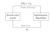
To state it more formally, our goal here will be to find a parameter \(\theta^*\) such that
\[ \theta^* \in \arg\min_{\theta} f(\theta), \tag{1.1} \]
given noisy samples or observations of the performance objective \(f\). As illustrated in Figure 1.1, an iterative optimization algorithm queries the zeroth-order oracle for the objective value at the parameter \(\theta_n\) at time instant \(n\), and receives the observation \(f(\theta_n) + \xi_n\). Here \(\xi_n\), \(n\geq 1\) is a sequence of ‘noise’ random variables. For instance, as we consider in this book, this sequence could be a martingale difference sequence. It is important to note here that the noisy observations \(f(\theta_n)+\xi_n\) above cannot be separated into the objective function value \(f(\theta_n)\) and the noise component \(\xi_n\) to infer the form of the objective function directly from the given noise corrupted data. Thus, it is assumed that the noisy data samples are obtained either from a simulation device or a real system. The obtained data is then used by the optimization algorithm. Since we do not estimate the objective function \(f\) and yet run the optimization procedure using only noisy samples, we many times refer to techniques that solve such problems as model-free optimization methods. On the contrary, approaches that are based on estimating the function \(f\) are called model-based optimization techniques. The performance value \(f(\theta)\) and the sample performance \(g(\theta,\xi) = f(\theta)+\xi\) are related as \(f(\theta) = E[g(\theta,\xi)]\), where \(E[\cdot]\) denotes the expectation w.r.t the distribution of \(\xi\). It is assumed here that the noise random variable \(\xi\) has a mean of zero.
Note also that (1.1) contains ‘\(\in\)’ instead of ‘\(=\)’. This is because the minimizer need not be unique and so \(\arg\min_\theta f(\theta)\) would constitute the set of all parameters \(\theta\) that attain the minimum. The set is a singleton if the minimizing parameter is unique. In general, finding one of the minimizers is sufficient in such problems. However, it is important to observe that finding a global minimum, in this setting, is far more computationally intensive than finding a local minimum. In this book, we shall focus on solution methods that aim at finding a local minimum. In most applications, the minima are also isolated in the sense that around any minimum, one can draw a ball of a small enough radius such that it contains only the given (and no other) minimum.
1.2 Applications
Several real-world systems in disciplines such as communication networks, healthcare, finance, are too complex to directly optimize among a set of choices. A viable alternative is to build a simulator for various components of the system, and then perform the optimization over decisions or choices via simulator access. Simulation optimization refers to this setting, where the goal is to find the optimum choice for a certain design parameter. For a given parametric description of the system, performance evaluations using the simulator are typically noisy (i.e., have a spread or distribution), and each simulation to obtain an evaluation is often computationally expensive. Thus, in addition to searching for optima, a good simulation optimization algorithm should ensure that the number of function evaluations is small.
Simulation optimization falls under the realm of zeroth-order optimization, and gradient-based algorithms are efficient solution alternatives for finding an optimum using observations from a simulator. The reader is referred to (Fu 2015) for a detailed introduction to simulation optimization. For a survey of simulation software catering to a variety of applications, see (Swain 2017).
An area of practical interest for zeroth-order optimization algorithms is reinforcement learning (RL) (R. S. Sutton and Barto 2018; D. P. Bertsekas and Tsitsiklis 1996; D. Bertsekas 2019; Meyn 2022). In a typical RL setting, the goal is to maximize the cumulative reward over time by learning an optimal policy to choose actions. The underlying formalism is of a Markov decision process (MDP), where the algorithm interacts with the environment through actions, and as a response the environment changes its state and provides a reward. In an MDP, the next state depends on the current state and the chosen action.
Policy gradient methods (Richard S. Sutton et al. 1999; Konda and Tsitsiklis 2003; S. Bhatnagar et al. 2009) are a popular solution approach for such problems. The basis for such algorithms is the policy gradient theorem, which motivates the use of likelihood ratio based gradient estimates. While such an approach of obtaining unbiased gradient estimates works in a risk-neutral RL setting, the same is not true if one incorporates a risk measure in the problem framework. As an example, one could modify the problem to find a policy with the highest mean cumulative discounted reward, while imposing a constraint on the variance. In such a setting, it is difficult to employ the likelihood ratio method for estimating gradient, and simultaneous perturbation methods, which we discuss in detail in this book, are a viable alternative. In (Prashanth and Ghavamzadeh 2016), the authors employ such an approach to find a risk-optimal policy, which handles a mean-variance tradeoff. Moreover, in (Vijayan and Prashanth 2021), the authors show that a policy gradient algorithm employing the simultaneous perturbation method for gradient estimation performs on par with REINFORCE — an algorithm that uses the likelihood ratio method for gradient estimation.
More generally, zeroth order optimization approaches have been found useful in the context of simulation optimization under inequality constraints (Shalabh Bhatnagar, Hemachandra, and Mishra 2011), actor-critic algorithms which are RL algorithms based on the policy iteration procedure (Shalabh Bhatnagar and Kumar 2004; Abdulla and Bhatnagar 2007), simulation-based algorithms for finding optimal policies in finite horizon MDPs (Shalabh Bhatnagar and Abdulla 2008), RL algorithms for constrained MDPs (Shalabh Bhatnagar 2010; Shalabh Bhatnagar and Lakshmanan 2012), as well as discrete parameter simulation optimization (Gerencser, Hill, and Vago 1999; Shalabh Bhatnagar, Mishra, and Hemachandra 2011). In (Shalabh Bhatnagar et al. 2006), the problem of finding the optimal policy in an MDP setting conditioned on a rare event is considered and a zeroth order simulation optimization algorithm is presented and analysed. It is shown that the resulting scheme has close connections with risk sensitive MDPs with exponentiated costs. In most of the aforementioned settings, it is not easy to obtain likelihood ratio based sample gradient estimates, hence application of zeroth order methods becomes inevitable.
A more recent application of zeroth-order optimization algorithms, of the type discussed in this book, is in the context of large language models (LLMs), which are nearly ubiquitous, with widespread adoption across various disciplines. Traditional methods for LLM tuning involve high compute costs. To reduce the computational burden of LLM tuning, zeroth-order optimization methods have been explored recently, cf. (Malladi et al. 2023). This approach is less compute-intensive compared to a traditional backpropagation scheme with the well-known ADAM step-size schedule.
Adversarial machine learning is another recent application, where zeroth-order optimization techniques have been applied successfully to construct black-box adversarial examples, cf. (Ilyas et al. 2018; P.-Y. Chen et al. 2017; Bhagoji et al. 2018; Ilyas, Engstrom, and Madry 2019; Alzantot et al. 2019; J. Chen, Jordan, and Wainwright 2020; Mukhoty et al. 2023; Dong et al. 2020). The idea here is to use zeroth-order gradient estimates, similar to SPSA discussed earlier, to approximate the gradient of a target neural network, and use this model to general adversarial images that lead to misclassification. Such adversarial examples are concerning from a security viewpoint, in a safety critical application such as autonomous driving. Zeroth-order gradient estimates have also been employed to make machine learning models robust during training, see (Zhang et al. 2022).
1.3 Stochastic approximation algorithms
The algorithms that we shall present here are all going to be of the stochastic approximation type. The basic stochastic approximation scheme, also referred to as the Robbins-Monro algorithm, named after its inventors, H.Robbins and S.Monro, see (Robbins and Monro 1951), was designed to find the zeros of an unknown function \(h:\mathbb{R}^d\rightarrow\mathbb{R}^d\). The algorithm tunes up the parameter values incrementally based on noisy observations of the function \(h\) obtained using the most recent parameter values as they become available. The basic stochastic approximation scheme has the following form:
\[ \theta_{n+1} = \theta_{n} + a(n) (h(\theta_{n}) + \xi_n), \tag{1.2} \]
starting from an initial parameter estimate \(\theta_0 \in \mathbb{R}^d\). Here, \(a(n),n\geq 0\) is the step-size sequence of positive real numbers. Given the parameter update \(\theta_{n}\) at the \(n\)th epoch, a noise-corrupted measurement \(h(\theta_{n})+\xi_n\) of the objective is obtained and used to update the parameter \(\theta_{n}\) to obtain a new parameter \(\theta_{n+1}\) according to (1.2). As can be seen, smaller step sizes while reducing the noise effects result in more graceful albeit slower convergence. On the other hand, larger step sizes result in faster tracking of the function’s zeros though at the cost of higher variance in the iterates. A crucial aspect is one of ensuring convergence that would result in the desired outcome. This and other related aspects will be made more precise in later chapters.
Typical applications of stochastic approximation algorithms include finding the fixed points of a function whose noisy estimates alone are available, as well as finding a minimum of a function again under noisy observations. In the former case, \(h(\theta)\) in (1.2) can have the form \(h(\theta) = g(\theta)-\theta\) for some function \(g:\mathbb{R}^d \rightarrow \mathbb{R}^d\), while in the latter, \(h(\theta)\) can be of the form \(h(\theta) = -\nabla f(\theta)\) for some function \(f:\mathbb{R}^d\rightarrow \mathbb{R}\). The gradient form of the objective will be of interest to us here except that we will assume that just like the objective function, even the gradient is also not known analytically to us. Noisy function measurements will be used to estimate the gradient. We shall also present some recent Hessian estimation approaches in addition to gradient estimation procedures that will be used in noisy Newton-based schemes. We shall see that one may write the noisy gradient scheme involving gradient estimates as
\[ \theta_{n+1} = \theta_{n} + a(n) (-\nabla f(\theta_{n}) + \xi_n + \eta_n). \tag{1.3} \]
Here \(h(\theta_{n})\) in (1.2) is replaced with \(-\nabla f(\theta_{n})\). However, the important difference is that there is an extra error term \(\eta_n\) in (1.3) that is however not present in (1.2). This error arises because of the gradient estimates obtained from noisy function measurements.
The original Robbins-Monro algorithm was aimed at solving the root finding problem under noisy observations of the function objective with the noise random variables assumed to be forming an independent and identically distributed (i.i.d) sequence. Under certain conditions, convergence was shown in (Robbins and Monro 1951) to the root of the desired system of equations in the mean-squared sense. Kiefer and Wolfowitz developed a stochastic approximation algorithm to find the maximizer of a given objective function, see (Kiefer and Wolfowitz 1952). We shall discuss this algorithm in more detail in the next section as indeed this was the first zeroth-order stochastic optimization algorithm and used a finite-difference gradient estimates derived from noisy function measurements. As with (Robbins and Monro 1951), the objective function in (Kiefer and Wolfowitz 1952) was considered to be a regression function. The iterate-sequence was shown to converge in probability to the optimum. In (R.Blum 1954), weaker conditions were developed to ensure that both Robbins-Monro and Kiefer-Wolfowitz algorithms converge with probability one to the desired equilibria. In (A.Dvoretzky 1956), a more general objective function was considered and under weaker conditions both mean-squared convergence and convergence with probability one were shown.
In another major development, the ordinary differential equation (ODE)-based analysis of stochastic approximation algorithms was introduced by (Ljung 1977) and (Kushner and Clark 1978). It was shown that under certain conditions, one may study the asymptotic behavior of a stochastic approximation algorithm by analyzing the same for an associated ODE. The ODE associated with (1.2) can be seen to correspond to
\[ \dot{\theta}(t) = h(\theta(t)). \tag{1.4} \]
The main result of (Ljung 1977) and (Kushner and Clark 1978) would say the following:
The above corresponds to a strong notion of recurrence for the ODE, and may not be applicable in many situations. In (Benaïm 1996), (Benaïm 1999) and (Benaïm and Hirsch 1996), the ODE based analysis of (Ljung 1977) and (Kushner and Clark 1978) has been extended to the setting where the asymptotic behavior of the algorithm is analyzed via a weaker notion of recurrence, namely chain recurrence, of the underlying ODE. Most of the modern ODE based analyses follow the latter approaches.
1.4 Zeroth-order stochastic gradient (SG) algorithm
Consider the following stochastic approximation scheme:
\[ \theta_{n+1} = \theta_{n} + a(n) (-\widehat{\nabla} f(\theta_{n})), \tag{1.5} \]
where \(\widehat{\nabla}f(\theta_{n})\) is a noisy estimate of the gradient of \(f(\theta_{n})\), with \(f:\mathbb{R}^d\rightarrow\mathbb{R}\) being the objective function to be minimized. The Kiefer-Wolfowitz scheme, see (Kiefer and Wolfowitz 1952), estimates the gradient \(\nabla f(\theta)\) using the following estimator: For \(i=1,\ldots, d\),
\[ \widehat{\nabla}_if(\theta_{n}) = \frac{1}{2\delta} \left(f(\theta_{n}+\delta e_i)+\xi^+_i(n) - f(\theta_{n}-\delta e_i)-\xi^-_i(n) \right), \tag{1.6} \]
\[ = \frac{1}{2\delta} \left(\left(f(\theta_{n}+\delta e_i)- f(\theta_{n}-\delta e_i)\right) + \left(\xi^+_i(n)-\xi^-_i(n)\right) \right), \]
where, \(\widehat{\nabla}_if(\theta_{n})\) denotes the estimate of the \(i\)th partial derivative of \(f(\theta_{n})\). Further, \(e_i =(0,\ldots,0, 1, 0,\ldots, 0)^T\) is the unit \(d\)-dimensional vector with 1 as the \(i\)th place and all other entries as 0. Further, \(\xi^+_i(n)\) (resp. \(\xi^-_i(n)\)) is the noise associated with the estimate of the function \(f\) measured at the parameter value \((\theta_{n}+\delta e_i)\) (resp. \((\theta_{n}-\delta e_i)\)).
Notice that in (1.6), assuming the function \(f\) to be sufficiently smooth, a first order Taylor’s expansion would lead to
\[ \frac{f(\theta_{n}+\delta e_i)- f(\theta_{n}-\delta e_i)}{2\delta} = \nabla_i f(\theta_{n}) + O(\delta^2). \]
This happens because the first and the third terms in the Taylor’s expansion get canceled as a consequence of the balanced nature of the estimate. The term comprising \(O(\delta^2)\) contributes to the bias in the gradient estimate. In relation to (1.3), if \(\delta\rightarrow 0\) as \(n\rightarrow \infty\) above, the analysis turns out to be a simple extension of the corresponding analysis for (1.2), see Chapter 2 of (Borkar 2022). However, letting the \(\delta\)-parameter approach zero results in constraining the choice of the step-size sequence \(\{a(n)\}\). Nonetheless, the recursion in such a case can be shown to track the ODE
\[ \dot{\theta}(t)=-\nabla f(\theta(t)). \tag{1.7} \]
For a fixed \(\delta>0\), on the other hand, it can be shown that for an algorithm as in (1.5) with say the Kiefer-Wolfowitz gradient estimator (1.6), given \(\epsilon >0\), \(\exists \delta_0>0\), such that when the ‘perturbation parameter’ \(\delta \in (0,\delta_0]\), the term \(\eta_n\) is \(O(\epsilon)\). Analyses with a fixed \(\delta\) can be carried out by viewing the resulting algorithm as one involving a set-valued map \(H(\theta)=\nabla f(\theta) + \bar{B}(0,\epsilon)\), where \(\bar{B}(0,\epsilon)\) is a closed ball of radius \(\epsilon\) around the origin. The resulting scheme can then be analysed by viewing the limiting system as the Differential Inclusion (DI)
\[ \dot{\theta}(t) \in -H(\theta(t)), \tag{1.8} \]
see, for instance, (Ramaswamy and Bhatnagar 2018).
A disadvantage with the gradient estimator defined above is that it requires \(2d\) function measurements or simulations to run one update of the parameter according to (1.5). The amount of computation thus can be very high for a large value of \(d\). In (James C. Spall 1992), the following estimator of the gradient has been proposed that uses only two function measurements regardless of the value of \(d\).
\[ \widehat{\nabla}_if(\theta_{n}) = \frac{f(\theta_{n}+\delta \Delta(n))+\xi^+(n) - f(\theta_{n}-\delta \Delta(n))-\xi^-(n)}{2\delta\Delta_i(n)}. \tag{1.9} \]
Here, \(\Delta(n)=(\Delta_1(n),\ldots,\Delta_d(n))^T\) is a vector of i.i.d random variables \(\Delta_j(n)\), \(j=1,\ldots,d, n\geq 0\) that are typically zero-mean with a finite inverse moment bound. Independent symmetric Bernoulli random variables such as \(\Delta_j(n) = \pm 1\) w.p. \(1/2\) are commonly used here. A Taylor’s expansion as with the Kiefer-Wolfowitz estimator would give the following in this case:
\[ \begin{align*} &\frac{f(\theta_{n}+\delta \Delta(n))- f(\theta_{n}-\delta \Delta(n))}{2\delta\Delta_i(n)} = \frac{\Delta(n)^T\nabla f(\theta_{n})}{\Delta_i(n)} +O(\delta^2) \\ &= \nabla_i f(\theta_{n}) + \sum_{j\not=i} \frac{\Delta_j(n) \nabla_j f(\theta_{n})}{\Delta_i(n)} + O(\delta^2). \tag{1.10} \end{align*} \]
Note the presence of an extra (the second) term on the RHS that contributes to the bias. It may however be observed that
\[ E\left[\sum_{j\not=i} \frac{\Delta_j(n) \nabla_j f(\theta_{n})}{\Delta_i(n)}\mid \theta_{n} \right] = 0. \]
It can therefore be seen that
\[ \begin{align*} \norm{ \EE{\widehat\nabla f(\theta_n) \mid \theta_n} \!-\! \nabla f(\theta_n) } \le C\delta^2, \tag{1.11} \end{align*} \]
for some positive scalar \(C\).
Since this estimate of \(\nabla f\) is used in the recursion (1.5), a stochastic approximation scheme, one recovers the expectation in the asymptotic limit of the iterate sequence as the noise effects die down. A one-simulation estimator was proposed in (James C. Spall 1997) where the form of the estimator was simply
\[ \widehat{\nabla}_if(\theta_{n}) = \frac{f(\theta_{n}+\delta \Delta(n))+\xi^+(n)}{\delta\Delta_i(n)}, \mbox{ }i=1,\ldots,d. \tag{1.12} \]
A Taylor’s expansion on the function value without the noise term in (1.12) gives
\[ \frac{f(\theta_{n}+\delta \Delta(n))}{\delta\Delta_i(n)} = \frac{f(\theta_{n})}{\delta\Delta_i(n)} + \nabla_if(\theta_{n}) + \sum_{j\not=i} \frac{\Delta_j(n) \nabla_j f(\theta_{n})}{\Delta_i(n)} + O(\delta). \]
The third term on the RHS above is the same as a corresponding term that contributes to the bias in (1.10). However, there is an additional first term on the RHS that also has zero mean given the parameter update \(\theta_{n}\). The latter term, however, is primarily responsible for below par performance of this estimate because of the presence of \(\delta\), a typically small quantity, in the denominator. The aforementioned estimators are popularly referred to as two-measurement and one-measurement simultaneous perturbation stochastic approximation (SPSA) estimators.
Deterministic perturbation versions of the above algorithms have been proposed in (Shalabh Bhatnagar et al. 2003) and are seen to yield better performance particularly for the one-simulation estimators when compared with their random perturbation counterparts. This is because of a regular (cyclic) cancellation of the previously mentioned bias terms when deterministic perturbation schedules are used. In other work along similar lines, the smoothed functional estimators have been studied in (Rubinstein 1981), (Katkovnik and Kulchitsky 1972), (Shalabh Bhatnagar and Borkar 2003), (S. Bhatnagar 2007), (S. Bhatnagar, Prasad, and Prashanth 2013), where the underlying perturbation distributions are primarily Gaussian, uniform and Cauchy. In (Ghoshdastidar, Dukkipati, and Bhatnagar 2014b, 2014a), smoothed functional algorithms with q-Gaussian perturbations have been presented that are seen to significantly extend the class of perturbations and allowing for a continuum of distributions depending on the value of the q-parameter.
Random directions stochastic approximation (RDSA) algorithm has been presented in (Kushner and Clark 1978) where the underlying distribution has been considered to be uniform on the surface of a sphere that is akin to the multivariate Gaussian distribution. In (Prashanth et al. 2017), algorithms with i.i.d., uniformly distributed perturbations have been proposed. These perturbations lie within a \(d\)-dimensional cube. Further, in (Prashanth et al. 2020), deterministic perturbation versions of these algorithms have been studied and analyzed. We shall be discussing some of these algorithms in more detail in a later chapter.
1.5 Zeroth-order stochastic Newton (SN) algorithm
Recall that a SG algorithm involves the following recursion:
\[ \begin{align*} \theta_{n+1} = \theta_n - a(n) \widehat\nabla f(\theta_n), \tag{1.13} \end{align*} \]
where \(\widehat\nabla f(\theta_n)\) is an estimate of the gradient \(\nabla f(\theta_n)\).
There are three main shortcomings in employing a SG algorithm. First, from an asymptotic convergence rate analysis (cf. (Fabian 1968)), it is apparent that the SG algorithm would achieve an order \(O\left(\frac{1}{\sqrt{n}}\right)\) convergence when the stepsize is set using the curvature of \(f\), i.e., \(a_n = a_0/n\) with \(a_0 > \delta/2\lambda_{\min}(\nabla^2 f(\theta^*))\). In practice, such curvature information is seldom available, and hence, it is problematic to assume such knowledge in setting the step-size for optimal convergence speed. Second, it is widely observed empirically that a SG algorithm declines fast initially, but slows down towards the end, i.e., when the SG iterate is near an optimum \(\theta^*\). Third, the update rule (1.13) is not scale-invariant, i.e., changing \(\theta\) to \(B\theta\) for some matrix \(B\), would imply a change in the update (1.13). Finally, a SG algorithm may get stuck in traps or unstable equilibria such as local maxima and saddle points, while the goal is for it to converge to local minima (esp. since convexity is not assumed).
A second-order SN algorithm overcomes the shortcomings of a first-order SG algorithm mentioned above. A general gradient-search algorithm involves an update rule of the form:
\[ \begin{align*} \theta_{n+1} = \theta_n - a(n) B(\theta_n)^{-1} \nabla f(\theta_n), \tag{1.14} \end{align*} \]
where \(B(\theta)\) for any \(\theta\in \mathbb{R}^d\) is a \(d\times d\) matrix. The following choices of the \(B(\theta)\) matrix are widely popular (see (Dimitri P. Bertsekas 1999)):
\(B(\theta)=I\) (the identity matrix) for all \(\theta\): In this case, the algorithm (1.14) reduces to the first-order SG algorithm (1.13).
\(B(\theta)\) is a diagonal matrix with diagonal entries being \(\nabla_{i,i}^2 f(\theta)\). This corresponds to the (second-order) Jacobi algorithm.
\(B(\theta) =\nabla^2 f(\theta)\): This corresponds to the second-order SN algorithm.
In the following, we focus on the SN algorithm (corresponding to the full Hessian case). As illustrated in Figure 1.2, the update rule above then requires computation of the Hessian as well as the gradient estimate at any parameter update \(\theta_n\).
We elaborate on the advantages of such an algorithm over the first-order scheme in (1.13) (or alternatively the case of \(B(\theta)=I\) in (1.14)). First, such algorithms achieve the optimum speed of convergence without the knowledge of \(\lambda_{\min}(\nabla^2 f(\theta^*))\). Setting \(a_0=1\) would suffice. Second, it is generally observed that second-order methods exhibit faster convergence in the final phase, i.e., when the iterates are close to the optima. This can be attributed to the fact that second-order methods minimize a quadratic model of \(f\), while SG algorithm (1.13) uses a first-order Taylor’s approximation. Third, second-order algorithms are scale-invariant, i.e., they auto-adjust to the scale of \(\theta\). Finally, second-order algorithms avoid traps naturally, since they factor in curvature information through the Hessian. On the flip side, second-order methods have a higher per-iteration cost than their first-order counterparts, as the Hessian matrix has to be inverted during each iteration.
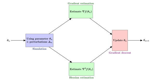
In the zeroth-order optimization setting that we consider, we do not have direct access to the gradient and the Hessian of the objective function. Instead, as illustrated in Figure 1.2, both gradient and Hessian have to estimated from noisy function observations before performing a parameter update. In other words, letting \(\widehat \nabla f(\theta_n)\) and \(\overline{H}_n\) denote the gradient and Hessian estimates, we update the parameter as follows:
\[ \begin{align*} \theta_{n+1} = \theta_n - a(n) \left( \overline{H}_n\right)^{-1} \widehat\nabla f(\theta_n). \tag{1.15} \end{align*} \]
The topic of gradient estimation is handled in Chapter 3, while Chapter 6 focuses on Hessian estimation, and the convergence analysis of (1.15), where we use zeroth-order estimates of both the gradient and the Hessian.
To understand the problem of Hessian estimation, we now discuss a finite difference approximation, which requires \(O(d^2)\) function measurements. The simultaneous perturbation trick brings this number down to a small constant, regardless of the parameter dimension \(d\). We shall discuss these schemes in detail in Chapter 6.
Consider a scalar variable \(\theta\). A finite difference approximation of the first derivative for this simple case of a scalar parameter \(\theta\) is:
\[ \begin{align*} \frac{d f(\theta)}{d\theta} \approx \left(\dfrac{ f(\theta+\delta) - f(\theta-\delta)}{2\delta}\right). \tag{1.16} \end{align*} \]
Assuming the objective is smooth, and employing Taylor series expansions of \(f(\theta+\delta)\) and \(f(\theta-\delta)\) around \(\theta\), we obtain:
\[ \begin{align*} f(\theta\pm\delta) &= f(\theta) \pm \delta \frac{d f(\theta)}{d\theta} + \frac{\delta^2}{2} \frac{d^2 f(\theta)}{d\theta^2} + O(\delta^3), \\ \text{Thus, }\dfrac{ f(\theta+\delta) - f(\theta-\delta)}{2\delta} &= \dfrac{d f(\theta)}{d\theta} + O(\delta^2). \end{align*} \]
From the above, it is easy to see that the estimate (1.16) converges to the true gradient \(\dfrac{d f(\theta)}{d\theta}\) in the limit as \(\delta \rightarrow 0\).
This idea can be extended to estimate the second derivative by applying a finite difference approximation to the derivative in (1.16) as follows:
\[ \begin{align*} &\frac{d^2 f(\theta)}{d\theta^2} \approx \\ &\quad\frac{\left(\dfrac{ f(\theta+\delta + \delta) - f(\theta + \delta - \delta)}{2\delta}\right) - \left(\dfrac{ f(\theta - \delta + \delta) - f(\theta-\delta - \delta)}{2\delta}\right)}{2\delta} \tag{1.17} \end{align*} \]
As before, using Taylor series expansions, it can be shown that the RHS above is a good approximation to the second derivative.
For the case of a vector parameter, one needs to perturb each co-ordinate separately, leading to the following scheme for estimating the Hessian \(\nabla^2 f(\theta)\): For any \(i,j \in \{1,\ldots,d\}\),
\[ \begin{align*} \nabla^2_{ij} f(\theta) &\approx \frac{1}{4\delta^2}\bigg( f(\theta+\delta e_i + \delta e_j) + f(\theta+\delta e_i - \delta e_j) \\ &\qquad\qquad - \left( f(\theta-\delta e_i + \delta e_j) - f(\theta-\delta e_i - \delta e_j)\right)\bigg). \tag{1.18} \end{align*} \]
Such an approach requires \(4d^2\) number of function measurements to form the Hessian estimate. In the next section, we overcome this limitation by employing the simultaneous perturbation trick. Before that, we extend the estimate in (1.18) to the noisy case as follows: Suppose we have the following function measurements: For any \(i,j \in \{1,\ldots,d\}\),
\[ \begin{align*} &y_{1} = f(\theta+\delta e_i + \delta e_j) + \xi_{1ij}, y_{2} = f(\theta+\delta e_i - \delta e_j) + \xi_{2ij}, \tag{1.19} \\ &y_{3} = f(\theta-\delta e_i + \delta e_j) + \xi_{3ij} \textrm{ and } y_{4} = f(\theta-\delta e_i - \delta e_j)+ \xi_{4ij}. \tag{1.20} \end{align*} \]
Using these function measurements, we form the Hessian estimate \(\widehat H\) as follows:
\[ \begin{align*} \widehat H_{ij} & = \left(\dfrac{y_1 - y_2 - y_3 + y_4}{4\delta^2}\right), \forall i,j \tag{1.21} \end{align*} \]
Assuming the function is sufficiently smooth, as in the gradient case and the noise elements in the function measurements are zero mean, it can be shown through Taylor series expansions that
\[ \begin{align*} \E[\widehat H_{ij} \mid \theta] &= \frac{1}{4\delta^2}\bigg( f(\theta+\delta e_i + \delta e_j) + f(\theta+\delta e_i - \delta e_j) \\ &\qquad\qquad - \left( f(\theta-\delta e_i + \delta e_j) - f(\theta-\delta e_i - \delta e_j)\right)\bigg) \\ & = \nabla^2_{ij} f(\theta) + O(\delta^2). \end{align*} \]
While the bias of the estimator is on the lower side, with explicit control via the \(\delta\) parameter, the problem is in the number of function measurements. The latter number is \(4d^2\), limiting the practical viability on high-dimensional problems. In Chapter 6, we discuss several alternative schemes using the simultaneous perturbation method for Hessian method. These schemes use a small (constant) number of function measurements (regardless of the parameter dimension \(d\)), while ensuring a bias of \(O(\delta^2)\).
1.6 Organization of the book
We now describe the organization of the rest of the book.
In Chapter 2, we provide an introduction to stochastic approximation algorithms, and outline a few popular applications such as mean estimation, gradient-type algorithms, fixed-point iterations, and quantile estimation. These algorithms are incremental update procedures that work with stochastic or noisy data as it becomes available and are model-free procedures. In Chapter 2, we provide a detailed introduction to stochastic approximation algorithms, provide motivating applications, and subsequently provide the main results on convergence of these schemes. It turns out that many of the stochastic optimization schemes require a treatment of algorithms with set-valued maps. We also present such algorithms in settings where data samples become available one at a time in real time, and so are Markovian. We therefore discuss the main convergence results in connection with these as well. In addition, Newton-based stochastic optimization schemes involve estimating the inverse of the Hessian of the objective. This cannot be done using the standard stochastic approximation template and we need such algorithms to perform updates using two-timescale procedures. We therefore also discuss two-timescale stochastic approximation algorithms (including those with set-valued maps) in this chapter.
In Chapter 3, we provide a variety of gradient estimators using the simultaneous perturbation method. These include unified two-point as well as one-point gradient estimation schemes. The unified estimates feature abstract random perturbations that are required to satisfy certain conditions to ensure that the bias and variance of the estimates is manageable. Specializing these estimates with specific choice of random perturbations leads to several well-known simultaneous perturbation-based schemes such as the smoothed functional scheme (Katkovnik and Kulchitsky 1972) with later refinements in (Polyak and Tsybakov 1990; Dippon 2003; Nesterov and Spokoiny 2017), random direction stochastic approximation (RDSA) scheme proposed by (Kushner and Clark 1978), and recently enhanced in (Prashanth et al. 2017), and the popular simultaneous perturbation stochastic approximation (SPSA) scheme proposed by (James C. Spall 1992). While most estimators that we present require one or two function measurements in order to estimate the gradient, we also touch upon a recently developed class of generalized simultaneous perturbation gradient estimators that provide estimators requiring a number of function measurements that depends on the bias in the gradient estimator. We analyze the bias and variance of the aforementioned estimators in the convex as well as the non-convex regimes. In either case, the analysis requires the objective to be smooth.
In Chapter 4, we present a detailed mathematical treatment of a stochastic gradient algorithm that employs simultaneous perturbation-based gradient estimates. In particular, we cover asymptotic convergence of the stochastic gradient scheme using the popular ordinary differential equation (or ODE) method. It turns out that in many of these algorithms, it makes sense to hold the sensitivity parameter in the gradient estimation procedure fixed and not push it to zero in order that the estimator variance does not blow up. In such a case, we observe that the resulting scheme can be viewed as a stochastic recursive inclusion, i.e., one involving set-valued maps. Thus, we use here the theory of differential inclusions to establish that the stochastic gradient algorithm converges to a chain-recurrent set of an underlying differential inclusion.
In Chapter 5, we present the non-asymptotic analysis for the zeroth-order SG (ZSG) algorithm. In the case of a non-convex objective, we bound the expected decrease in the objective function in each iteration using the bias and variance properties of the gradient estimators together with a standard Taylor series argument. The expected decrease is used to provide an overall bound, which shows that the stochastic gradient algorithm converges to an approximate stationary point of the objective, with a rate \(O(\frac{1}{\sqrt{N}})\), where \(N\) is the number of iterations. In this chapter, we also analyze the rate of convergence of ZSG algorithm when the underlying objective is either convex or else strongly-convex. In the former case, we bound the optimization error (difference in function value between that of the iterate and the optimum), while in the latter case, we bound the parameter error, which is the norm of the distance between ZSG iterate and the optimum. Strong convexity allows a bound on the parameter error, while in the case of a non-strongly convex function, only a bound on the difference in function value is feasible. This is true even in the deterministic optimization setting, though the rates are slower in the stochastic zeroth-order setting that we study in this book. In this chapter, we also present a minimax lower bound using information-theoretic arguments, and this bound shows that the upper bounds for the ZSG algorithm are optimal up to a constant factor for the convex/strongly-convex cases.
In Chapter 6, we cover Hessian estimation using simultaneous perturbation methods. In particular, we provide a theoretical introduction to second-order SPSA proposed in (J. C. Spall 2000) as well as its later enhancements in (S. Bhatnagar 2005; S. Bhatnagar and Prashanth 2015). We also describe second-order smoothed functional (S. Bhatnagar 2007) and second-order RDSA (Prashanth et al. 2017) schemes. We analyze the bias in these Hessian estimates, and establish that each of these aforementioned schemes results in an asymptotically unbiased Hessian estimate. In this chapter, we also analyze a stochastic Newton algorithm using gradient/Hessian estimates based on the simultaneous perturbation method. As mentioned previously, these algorithms involve two-timescale stochastic approximation schemes. The theoretical guarantees that we provide include the asymptotic almost sure convergence of the stochastic Newton scheme, and an asymptotic normality result that can be used to bound the asymptotic covariance, which in turn helps one understand the mean-square error of the algorithm after a sufficiently large number of iterations. The latter analysis provides a convergence rate for the stochastic Newton algorithm, albeit in an asymptotic sense.
In Chapter 7, we focus on the points of convergence of the stochastic approximation schemes. An important consideration such algorithms is to ensure that the stochastic algorithm converges to local minima and not to saddle points that while being stationary points of the system, are in fact, unstable equilibria of the underlying ODE. Two schemes to escape saddle points are presented. In the first scheme, additional assumptions on the richness of noise are provided in the case of a general zeroth order gradient estimation scheme that would ensure avoidance of saddle points. We review these conditions on the noise from (Pemantle 1990) and provide the basic results. The second scheme deals with a cubic regularized Newton-based formulation from (Maniyar et al. 2024) with gradient and Hessian estimates obtained using zeroth-order estimation procedures. Convergence to an \(\epsilon\)-second order stationary point is then shown.
In Chapter 8, we provide applications of simultaneous perturbation methods in the reinforcement learning (RL) context. The first application involves a constrained discounted Markov decision process (MDP). In an RL setting, direct gradient measurements of the objective or value function are not available. Instead, one can estimate the value function using a Monte Carlo scheme, or the popular temporal difference (TD) learning algorithm. We consider the stochastic shortest path setting here. Assuming a smooth class of parameterized policies, we describe a policy gradient scheme that employs SPSA-based gradient estimates in conjunction with value function estimation using Monte Carlo samples as with the REINFORCE algorithm. We present a convergence analysis of our algorithm, which shows that the algorithm converges almost surely to local optima in the asymptotic limit. The second application considers a risk-sensitive RL problem, where the goal is to find a policy that maximizes the value function while satisfying a constraint that is formed using a risk measure. As in the first application, we describe a policy gradient algorithm for solving the risk-constrained MDP, and provide an asymptotic convergence analysis of this algorithm.
We also provide five appendices of useful background material. We outline the content of the appendices below.
Appendix A covers significant material on ODEs and differential inclusions, specifically from the viewpoint of stability, equilibria, attractors, as well as weaker notions of recurrence. These concepts are required for the asymptotic analysis of stochastic gradient and Newton algorithms in Chapters 2, 4 and 6, respectively.
Appendix B provides an introduction to selected topics in probability that are relevant to this book. In particular, we discuss various notions of convergence of random variables in this appendix. Next, we cover conditional expectation and provide a detailed introduction to martingales, including examples from stochastic approximation and asymptotic convergence results. The latter results on martingale convergence are useful in the analysis of stochastic approximation algorithms in general (see Chapter 2), and zeroth-order gradient-based algorithms in particular (see Chapters 4 and 6). To elaborate, stochastic gradient and Newton algorithms involve increments with a martingale difference noise sequence and it is important to understand when this sequence converges, so that an ODE or differential inclusions-based analysis of the aforementioned algorithms is feasible.
Appendix C provides an introduction to Markov chains in discrete time. This background is useful in understanding stochastic approximation algorithms with a Markovian noise component (see Section 2.6.
Appendix D provides foundational material on smooth optimization. In particular, first/second-order optimality conditions, smoothness and convexity are discussed in detail in this appendix.
Appendix E provides an introduction to information theoretic concepts such as entropy, and KL-divergence, followed by a statement with proof of a simpler version of the well-known Pinsker’s inequality. This background is useful for understanding the minimax lower bounds derived for a gradient-based algorithm with zeroth-order information in Section 5.6.
1.7 Bibliographic remarks
Kiefer and Wolfowitz in (Kiefer and Wolfowitz 1952) presented the first paper on stochastic gradient descent with zeroth order estimators and analysed their algorithm using the approach in (Robbins and Monro 1951). A comprehensive and detailed treatment of stochastic optimization including direct methods and evolutionary algorithms, in addition to zeroth order methods such as SPSA is available in (J. C. Spall 2005). A detailed treatment of stochastic simulation of random variables and processes including those driven by stochastic differential equations that also contains stochastic optimization is given in (Asmussen and Glynn 2007). Another textbook primarily on stochastic simulation that also deals with Markov chain Monte Carlo and discrete event system simulation, in addition to stochastic optimization (specifically, smoothed functional approaches) is (Rubinstein 1981).
A text that deals primarily with the theory of stochastic approximation is (Borkar 2022) that however also has a chapter on stochastic zeroth order methods for gradient estimation where methods such as SPSA and SF are briefly surveyed. Discrete event system simulation and optimization has been well-studied and analysed using perturbation analysis based methods in (Cassandras and Lafortune 2008). A text mainly dedicated to optimal control and reinforcement learning but which also delves a bit on zeroth order stochastic optimization is (Meyn 2022). A recent text on stochastic optimization and reinforcement learning covering a wide range of topics in these domains is (Powell 2021).
A textbook treatment of zeroth-order stochastic optimization approaches is available in (S. Bhatnagar, Prasad, and Prashanth 2013). The focus of the approaches presented in that text was to find the optimum parameter of an objective which in itself is a certain long-run average cost over noisy cost samples. A variety of methods for both unconstrained and constrained optimization including reinforcement learning are presented there. The resulting algorithms largely have a multi-timescale structure and the asymptotic convergence analysis of these algorithms is presented. In our current text, we primarily consider single-timescale stochastic optimization algorithms that estimate the gradient and (in some cases) the Hessian using zeroth order estimators though we also consider two-timescale algorithms for the latter case. We present newer and more general analyses of these algorithms and provide in detail both asymptotic as well as non-asymptotic convergence analyses of the presented algorithms. The asymptotic analyses are shown using limiting arguments involving underlying ordinary differential equations (ODE) or differential inclusions (with set-valued maps) as the case may be. Our current text also covers many recent algorithms not contained in (S. Bhatnagar, Prasad, and Prashanth 2013).