3 Gradient estimation
In this chapter, we introduce the simultaneous perturbation trick for gradient estimation, given noisy measurements from a zeroth-order oracle. These estimates are not unbiased, but feature a parameter that controls the bias, usually at the cost of variance. We discuss several popular gradient estimates in the literature, through a unified estimator. These estimates form the basis for a stochastic gradient algorithm, which is presented in Algorithm 1.
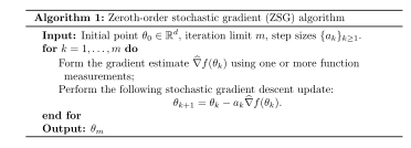
In the following section, we present schemes for devising \(\widehat\nabla f(\cdot)\) with an estimation error (bias) that can be made to vanish asymptotically. For the sake of analyzing the bias and variance properties of the gradient estimators in this chapter, we shall consider two classes of smooth functions, as given below. For a detailed introduction to smoothness, the reader is referred to Appendix D.
Definition 3.1.
Consider a function \(f:\R^d \rightarrow \R\).
- (i) \(f\) is \(L\)-smooth
-
if for some constant \(L > 0\),
\[ \| \nabla f ( x ) - \nabla f ( y ) \| \leq L \| x - y \|, \quad \forall x , y \in \mathbb { R } ^ {d }. \]
- (ii) \(f \in \cC^3\)
-
if \(f\) is three times continuously differentiable with
\(\left|\nabla^3_{i_1 i_2 i_3} f(\theta) \right| < \alpha_0 < \infty\), for \(i_1, i_2, i_3=1,\ldots, d\) and for all \(\theta\in \R^d\). Here \(\nabla^3 f(\theta) = \dfrac{\partial^3 f (\theta)}{\partial \theta\tr \partial \theta\tr \partial \theta\tr}\) denotes the third derivative of \(f\) at \(\theta\), and \(\nabla^3_{i_1 i_2 i_3} f(\theta)\) denotes the \((i_1 i_2 i_3)\)th entry of \(\nabla^3 f(\theta)\), for \(i_1, i_2, i_3=1,\ldots, d\).
3.1 Finite differences
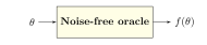
As a gentle start, consider a noise-free zeroth-order oracle, as illustrated below.
 {.book-asset fig-alt=” “}
In this setting, one could form an estimate \(\widehat\nabla f(\theta)\) using \(d+1\) queries to the oracle above as follows:
\[ \begin{align*} \widehat\nabla_i f(\theta) = \frac{1}{\delta} \left( f(\theta+\delta e_i) - f(\theta) \right)\,,\quad i=1,\dots,d\,. \tag{3.1} \end{align*} \]
How good an estimate is (3.1)? Assuming \(f\in \cC^3\), i.e., \(f\) is three-times continuously differentiable, we can employ Taylor series expansion of \(f\) as follows1:
\[ \begin{align*} f(\theta+ \delta e_i) &= f(\theta) + \delta\, \nabla f(\theta)^\top e_i + \frac{\delta^2}{2}\, e_i^\top \nabla^2 f(\theta) e_i + O(\delta^3), \end{align*} \]
leading to the estimation error:
\[ \begin{align*} \norm{ \widehat\nabla f(\theta) - \nabla f(\theta) } = O( \delta ). \end{align*} \]
Using \(2d\) queries to the oracle mentioned above, we define a two-sided variant of the estimate in (3.2) below.
\[ \begin{align*} \widehat \nabla_i f(\theta) = \frac{1}{2\delta} \left( f(\theta+\delta e_i) - f(\theta-\delta e_i) \right),\quad i=1,\dots,d. \tag{3.2} \end{align*} \]
Employing Taylor-series expansions as before, leads to the following bound on the estimation error:
\[ \begin{align*} \norm{ \widehat\nabla f(\theta) - \nabla f(\theta) } = O( \delta^2 ). \end{align*} \]
Thus, using a two-sided estimate reduced the error to \(O( \delta^2 )\), while the number of sample measurements went up to \(2d\) from \(d+1\).
The two estimates presented in (3.1) and (3.2) fall under the realm of finite difference stochastic approximation (FDSA), and such schemes can be extended to handle noise-corrupted function observations, as we show next. As an aside, a major disadvantage with FDSA estimates is the high measurement cost, since \(O(d)\) calls to the oracle are needed to form an estimate.
FDSA with noisy measurements
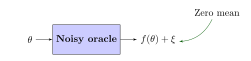
We consider a zeroth-order oracle, which outputs noisy observations of the objective at any query point, as illustrated below.
 {.book-asset fig-alt=” “}
Consider the following two-sided estimate, formed using noisy function measurements2:
\[ \begin{align*} \widehat\nabla_i f(\theta) = \frac{1}{2\delta} \left\{ f(\theta+\delta e_i) + \xi^+_i- (f(\theta-\delta e_i)+\xi^-_i) \right\},\quad i=1,\dots,d. \end{align*} \]
Suppose that \(\EE{\xi^{+} -\xi^- } = 0\) and also that \(\EE{ {\xi^{\pm}}^2 } \le \sigma^2 <\infty\). Then, assuming \(f\in \cC^2\), one can establish the near-unbiasedness of the estimate above using Taylor-series expansions as follows:
\[ \begin{align*} &f(\theta \pm \delta e_i) = f(\theta) \pm \delta\, \nabla f(\theta)^\top e_i + \frac{\delta^2}{2}\, e_i^\top \nabla^2 f(\theta) e_i + O(\delta^3). \\ &\Rightarrow \E( \widehat\nabla_i f(\theta) ) = \frac{1}{2\delta} \left( f(\theta+\delta e_i) - f(\theta-\delta e_i) \right) \\ &\Rightarrow \norm{ \E{\widehat\nabla f(\theta)} - \nabla f(\theta) } = O( \delta^2 ). \end{align*} \]
With \(2d\) queries, an FDSA estimate would be \(O(\delta^2)\) from the true gradient, even in the case when function measurements are noisy.
Next, we will present a series of estimates that achieve the same level of accuracy as FDSA, but with only two measurements, irrespective of the dimension \(d\).
3.2 Simultaneous perturbation method
FDSA perturbs co-ordinates one-at-a-time, leading to \(2d\) queries to the oracle. The number of queries get reduced by randomly perturbing all co-ordinate directions simultaneously. This is the idea behind the SPSA scheme proposed by (Spall 1992), which we describe below.
Let \(y^+ = f(\theta+\delta \Delta) + \xi^+\) and \(y^- = f(\theta-\delta\Delta) + \xi^-\), where \(\Delta = (\Delta_1,\ldots, \Delta_d)\tr\) is a \(d\)-vector of independent, symmetric, \(\pm 1\)-valued Bernoulli r.v.s, i.e., \(\Delta_i = +1\) w.p. \(1/2\) and \(-1\) w.p. \(1/2\), for \(i=1,\ldots,d\). It is important to mention that (Spall 1992) provides general conditions on the perturbation distribution and symmetric Bernoulli is a popular special case that we also consider here for simplicity. The gradient estimate here is given as follows:
\[ \begin{align*} \widehat\nabla_i f(\theta) = \left[ \dfrac{y^+ - y^-}{2\delta \Delta_i}\right],\,\, i=1,\ldots,d. \tag{3.3} \end{align*} \]
In expectation, the estimate defined above is nearly unbiased, and this can be argued as follows: Assuming \(\EE{\xi^+ - \xi^-} = 0\),
\[ \begin{align*} \EE{\widehat\nabla_i f(\theta)} = \EE{\dfrac{f(\theta + \delta \Delta) - f(\theta - \delta \Delta)}{2 \delta \Delta_i}}. \tag{3.4} \end{align*} \]
Here and in what follows, we assume that \(\theta\) is given, and the expectation is over other random terms.
Next, assuming \(f\in \cC^3\), and employing Taylor series expansions, we obtain
\[ \begin{align*} f(\theta \pm \delta \Delta) = f(\theta) \pm \delta \Delta\tr \nabla f(\theta) + \frac{\delta^2}{2}\, \Delta\tr \nabla^2 f(\theta) \Delta + O(\delta^3). \tag{3.5} \end{align*} \]
From the above, it is easy to see that
\[ \begin{align*} &\dfrac{f(\theta + \delta \Delta) - f(\theta - \delta \Delta)}{2 \delta \Delta_i} - \nabla_i f(\theta)=\underbrace{\sum_{j=1,j\not=i}^{d} \frac{\Delta_j}{\Delta_i}\nabla_j f(\theta)}_{(I)} + O(\delta^2). \end{align*} \]
In expectation given \(\theta\), term (I) above is zero, since \(\Delta_l, l=1,\ldots,d\) are independent, symmetric, Bernoulli \(\pm 1\)-valued r.v.s. Hence,
\[ \EE{\widehat\nabla_i f(\theta)} = \nabla_i f(\theta) + O(\delta^2). \]
From the above, it is easy to see that the expected value of the estimate (3.3) converges to the true gradient \(\nabla f(\theta)\) in the limit as \(\delta \rightarrow 0\). Thus, if one uses a gradient estimate as in (3.3) in a stochastic approximation algorithm, and lets \(\delta \rightarrow 0\) slowly enough, the overall scheme will converge to local minima of the function \(f\). This will be made precise in the next chapter.
We demonstrated the simultaneous perturbation trick through the SPSA scheme, which employed independent symmetric Bernoulli r.vs for random perturbations. As mentioned before, the trick is more generally valid and is not restricted to this choice of random perturbations alone. Furthermore, this trick can be used to estimate the Hessian, and not just the gradient, as we illustrate later.
In the next section, we present a unified gradient estimate that covers several schemes in the literature.
3.2.1 A unified estimate
Let \(y^+= f(\theta+\delta U)+\xi^+\), and \(y^- = f(\theta- \delta U)+\xi^-\). Using these function values, we form the gradient estimate as follows:
\[ \begin{align*} \widehat\nabla f(\theta) = \left(\frac{ y^+ - y^-}{2\delta}\right) V. \tag{3.6} \end{align*} \]
The estimate defined above can be specialized to cover several popular simultaneous perturbation-based gradient estimates, and we list some of these below.
Setting \(U \sim \cN(0,I_d)\), where \(\cN(0,I_d)\) denotes the \(d\)-dimensional standard Gaussian vector, and \(V = U\), we obtain the smoothed functional scheme proposed by (Styblinski and Tang 1990) (see also (Katkovnik and Kulchitsky 1972) for a one-sided variant). The latter scheme has been refined by (Polyak and Tsybakov 1990), and also studied by (Dippon 2003; Shalabh Bhatnagar and Borkar 2003; S. Bhatnagar 2007; Nesterov and Spokoiny 2017).
Setting \(U_i\) to be symmetric \(\pm 1\)-valued Bernoulli r.v.s and \(V = U\), we obtain the SPSA gradient estimate, which was defined earlier in (3.3).
\(U \sim \mathrm{Unif}(\mathbb{S}_N)\), i.e., \(U\) is chosen uniformly at random on the surface of a \(d\)-dimensional unit sphere, and with \(V =d U\), we obtain the random direction stochastic approximation (RDSA) scheme proposed by (Kushner and Clark 1978). A variant of the RDSA scheme with other choices for random perturbations is discussed next.
Setting \(U_i\) to be a uniformly distributed r.v. in \([-\eta,\eta]\), and \(V=\frac{3}{\eta^2} U_i\), leads to the 1RDSA-Unif variant of (Prashanth et al. 2017). On the other hand, setting \(U_i\) to be an asymmetric Bernoulli r.v., i.e., taking values \(-1\) and \(1+\varepsilon\) with probabilities \(\frac{1+\varepsilon}{2+\varepsilon}\) and \(\frac{1}{2+\varepsilon}\), respectively, and \(V_i=\frac{1}{1+\varepsilon} U_i\) leads to the 1RDSA-Asymber variant of (Prashanth et al. 2017). Here \(\varepsilon>0\) is a constant, usually set to a small value.
We make the following assumptions for analyzing the unified estimator presented above:
Assumption A3.1.
Let \(U,V\) be random \(d\)-vectors satisfying \(\EE{ V U^\top } = I\) and \(\EE{\norm{V}^2}< \infty\).
Assumption A3.2.
The noise factors \(\xi^\pm\) in (3.6) satisfy
\[ \begin{align*} \E[\xi^+-\xi^- |\, U,V] &= 0, \text{~~ and ~~} \E [ (\xi^{+} - \xi^-)^{2} |\, U, V] \le \sigma^2 <\infty\,. \tag{3.7} \end{align*} \]
Assumption A3.3.
The objective \(f\) satisfies
\[ \begin{align*} \sup_{\theta\in \R^d}\E [ f(\theta \pm \delta U)^{2}] \le B <\infty\,. \tag{3.8} \end{align*} \]
The result below provide bias and variance bounds for the unified estimate presented above.
Proposition 3.1.
Assume A3.1–A3.3, \(\EE{ \norm{V} \norm{U}^3 } < \infty\), and also that \(f\in\cC^3\), with \(\left|\nabla^3_{i_1 i_2 i_3} f(\theta) \right| < \tilde B < \infty\), for \(i_1, i_2, i_3=1,\ldots, d\) and for all \(\theta\in \R^d\). Then, the gradient estimate defined in (3.6) satisfies the following bounds for any given \(\theta\):
\[ \begin{align*} \norm{ \EE{\widehat\nabla f(\theta)} - \nabla f(\theta) } &\le C_1\delta^2, \textrm { and } \\ \EE{\norm{ \widehat\nabla f(\theta) - \EE{\widehat\nabla f(\theta)} }^2} &\le \frac{C_2}{\delta^2}, \end{align*} \]
where \(C_1 = \frac{\tilde B \EE{ \norm{V} \norm{U}^3 }}{6}\), and \(C_2 = \EE{\norm{V}^2}\left( \sigma^2+B^2\right)\).
From the result above, it is apparent that the sensitivity parameter \(\delta\) controls the bias-variance tradeoff, i.e., small values of \(\delta\) imply a low bias and high variance, while large values of \(\delta\) implies high bias and low variance in the gradient estimate.
Proof.
Notice that
\[ \begin{align*} \E[\widehat\nabla f(\theta)] = \E\left[V\, \dfrac{f(\theta+\delta U) -f(\theta-\delta U)}{2\delta} \right], \end{align*} \]
since \(\E\left[ V\left(\dfrac{\xi^+ - \xi^-}{2\delta}\right) \right]= 0\) from A3.2.
Since \(f\in C^3\), we have the following Taylor series expansion of \(f\) around \(\theta\):
\[ \begin{align*} f(\theta \pm \delta U) &= f(\theta) \pm\delta\, U\tr\,\nabla f(\theta) + \frac{\delta^2}{2}\, U\tr \nabla^2 f(\theta) U \\ &\quad\pm \frac{\delta^3}{6} \nabla^3 f(\tilde \theta^{\pm})(U \otimes U \otimes U), \tag{3.9} \end{align*} \]
where \(\otimes\) denotes the Kronecker product and \(\tilde \theta^+\) (resp. \(\tilde \theta^-\)) is on the line segment between \(\theta\) and \((\theta + \delta U)\) (resp. \((\theta - \delta U)\)).
Now,
\[ \begin{align*} \begin{split} \MoveEqLeft V\, \dfrac{f(\theta+\delta U) - f(\theta-\delta U)}{2\delta} \\ &= VU^{\tr} \, \nabla f(\theta) + \frac{\delta^2}{12} V \left(\nabla^3 f(\tilde \theta^+)+\nabla^3 f(\tilde \theta^-)\right)(U \otimes U \otimes U). \end{split} \tag{3.10} \end{align*} \]
Taking expectations of both sides above, using \(\EE{V U\tr} = I\), \(|\nabla^3 f(\tilde \theta^\pm)| < \tilde B\), and \(|\nabla^3 f(\bar\theta) (U \otimes U \otimes U)| \le \tilde B \norm{U}^3\) for any \(\bar\theta\), we obtain
\[ \begin{align*} \norm{ \EE{ \widehat\nabla f(\theta) } - \nabla f(\theta) } \le C_1\,\, \delta^2 \,, \textrm{ where }C_1 = \frac{\tilde B \EE{ \norm{V} \norm{U}^3 }}{6}. \end{align*} \]
Next, we prove the second claim concerning the variance of \(\widehat\nabla f(\theta)\). Notice that
\[ \begin{align*} &\E\left\| \widehat\nabla f(\theta) - \E \left[\widehat\nabla f(\theta)\right] \right\|^2 \le \E \left\|\widehat\nabla f(\theta) \right\|^2 \\ & = \E\left( \left\| V \right\|^2 \left(\left(\dfrac{\xi^+ - \xi^-}{2\delta}\right)^2 + 2 \left(\dfrac{\xi^+ - \xi^-}{2\delta}\right) \left(\dfrac{f(\theta+\delta U) - f(\theta-\delta U)}{2\delta}\right)\right.\right. \\ &\left.\left.\qquad\qquad+ \left( \dfrac{f(\theta+\delta U) - f(\theta-\delta U)}{2\delta} \right)^2 \right)\right) \\ &= \E\left( \left\| V \right\|^2 \left(\dfrac{\xi^+ - \xi^-}{2\delta}\right)^2\right) + 4 \E \left(\left\| V \right\|^2 \left( \dfrac{f(\theta+\delta U) - f(\theta-\delta U)}{2\delta} \right)^2\right) \tag{3.11} \\ & \le \frac{C_2}{\delta^2}\,, \end{align*} \]
where \(C_2 = \EE{\norm{V}^2}\left( \sigma^2+B^2\right)\). The equality in (3.11) follows from \(\EE{ \xi^+-\xi^- \,|\, U,V } = 0\).
\(\square\)
3.2.2 The convex case
We now analyze the bias and variance properties of the estimator in (3.6) under a convex objective \(f\). In this case, we do not require higher-order smoothness, and instead it is enough to assume first-order smoothness.
Proposition 3.2.
Assume A3.1–A3.3, \(\E[ \norm{V} \norm{U}^2]<\infty\), and also that the function \(f\) is convex and \(L\)-smooth, as specified in Definition 3.1. Then the gradient estimate defined in (3.6) satisfies the following bounds for any given \(\theta\):
\[ \norm{ \EE{\widehat\nabla f(\theta)} \!-\! \nabla f(\theta) } \le C_1\delta, \textrm { and } \EE{\norm{ \widehat\nabla f(\theta) - \EE{\widehat\nabla f(\theta)} }^2} \le \frac{C_2}{\delta^2}, \]
where \(C_1 \triangleq \dfrac{L}{2}\E[ \norm{V} \norm{U}^2]\) and \(C_2\) is as specified in Proposition 3.1.
Proof.
For any convex function \(f\) with an \(L\)-Lipschitz gradient, for any \(\delta>0\), it holds that
\[ \begin{align*} \frac{\<\nabla f(\theta), \delta u\>}{2\delta} \le \frac{f(\theta + \delta u) - f(\theta)}{2\delta} \le& \frac{\<\nabla f(\theta), \delta u\> + (L / 2) \norm{\delta u}^2}{2\delta}. \end{align*} \]
Using similar inequalities for \(f(\theta-\delta u)\), we obtain
\[ \begin{align*} \<\nabla f(\theta), u\> - \frac{L \delta \norm{ u}^2}{2} \le \frac{f(\theta + \delta u) - f(\theta-\delta u)}{2\delta} \le& \<\nabla f(\theta), u\> + \frac{L \delta \norm{ u}^2}{2}. \end{align*} \]
Letting \(\phi(\theta,\delta,u):=\frac1{\delta}\left(\frac{f(\theta + \delta u) - f(\theta-\delta u)}{2\delta} - \<\nabla f(\theta), u\>\right)\), we get
\[ \begin{align*} \left|\phi(\theta,\delta,u) \right| \le& \dfrac{L}{2} \norm{u}^2\,. \end{align*} \]
Using \(\EE{V U^\top}=I\) and A3.2, we obtain
\[ \begin{align*} \E[\widehat\nabla f(\theta)] &= \E\left[V\, \left(\frac{f(\theta+\delta U) -f(\theta-\delta U)}{2\delta}\right)\right] \\ &= \E\left[ V U^\top\nabla f(\theta) + \delta\phi(\theta,\delta,U) V \right] \\ &= \nabla f(\theta) + \delta \widehat\phi(\theta,\delta), \end{align*} \]
where \(\widehat\phi(\theta,\delta)\) satisfies \(\scnorm{\widehat\phi(\theta,\delta)} \le \, C_1 = \dfrac{L}{2}\E[ \norm{V} \norm{U}^2]\). The first claim concerning the bias of the gradient estimate follows.
The bound on the variance of the gradient estimate in (3.6) follows in a similar manner to the proof of Proposition 3.1.
\(\square\)
3.3 Variants
3.3.1 One-point gradient estimate
The gradient estimate presented earlier required two function evaluations. In this section, we describe a variant that requires only one function evaluation. Let \(y= f(\theta+\delta U)+\xi\). Using this function value, we form a gradient estimate as follows:
\[ \widehat\nabla f(\theta) = \frac{y}{\delta}V, \tag{3.12} \]
where \(U,V\) are random perturbations as in the case of two-point estimate (3.6), and \(\xi\) is a zero-mean noise r.v., i.e., satisfying \(\E[\xi|V]=0\).
Proposition 3.3.
Assume A3.1, A3.3, \(\EE{V} = 0\), and \(\E[\xi|V]=0\). Further, assume that \(U\) is symmetrically distributed, and \(V\) is an odd function of \(U\). Then, for \(f\in\cC^3\), the gradient estimate defined in (3.12) satisfies
\[ \norm{ \EE{\widehat\nabla f(\theta)} - \nabla f(\theta) } \le C_1\delta^2, \textrm { and } \EE{\norm{ \widehat\nabla f(\theta) - \EE{\widehat\nabla f(\theta)} }^2} \le \frac{C_2}{\delta^2}. \]
The \(O(\delta^2)\) bound on the bias above is comparable to the one obtained for the two-point estimate (3.6) in Proposition 3.1. However, a closer inspection of the proof reveals that the first and second term in the Taylor expansion (see (3.9)) cancel out in the case of the two-point estimate, while no such cancellation occurs in the one-point case. Instead, in the latter case, the corresponding Taylor terms turn out to be mean zero (see (3.13) in the proof below). Hence, the two-point estimate is preferable. Moreover, empirically the two-point estimate usually outperforms its one-point counterpart, as noted in (Spall 1997).
Proof.
Using \(\EE{ \xi|V}=0\), we have
\[ \begin{align*} \E[\widehat\nabla f(\theta)] = \E\left[ V \left(\dfrac{f(\theta+\delta U) }{\delta}\right)\right] \,. \end{align*} \]
By Taylor’s expansion in (3.9), we obtain
\[ \begin{align*} &\EE{V\, \dfrac{f(\theta+\delta U)}{\delta}} \\ &= \EE{V \frac{f(\theta)}{\delta}} + \EE{VU^{\tr} \, \nabla f(\theta)} + \EE{\frac{\delta}{2}\, V U\tr \nabla^2 f(\theta) U} \\ &\qquad+ \EE{\frac{\delta^2}{6} V \nabla^3 f(\tilde \theta^+)(U \otimes U \otimes U)} \\ &= \, \nabla f(\theta) + \EE{\frac{\delta^2}{6} V \nabla^3 f(\tilde \theta^+)(U \otimes U \otimes U)}. \tag{3.13} \end{align*} \]
The final equality above follows from the facts that \(\EE{V} = 0\), \(\EE{V U\tr} = I\) and for any \(i,j=1,\ldots,d\), \(E[V_i U_j^2] = 0\) since \(V\) is a deterministic odd function of \(U\), with \(U\) having a symmetric distribution. Using the fact that \(|\nabla^3 f(\tilde \theta^+) (U \otimes U \otimes U)| \le \tilde B \norm{U}^3\), we obtain
\[ \begin{align*} \norm{ \EE{ \widehat\nabla f(\theta) } - \nabla f(\theta) } \le C_1\,\, \delta^2 \,, \textrm{ where } C_1 = \frac{B_3 \EE{ \norm{V} \norm{U}^3 }}{6}. \end{align*} \]
The proof of the second claim concerning the variance of the estimate \(\widehat\nabla f(\theta)\) follows using arguments similar to those used in the proof of Proposition 3.1.
\(\square\)
3.3.2 Deterministic perturbations
So far, we have shown that one can use random perturbations to construct a gradient estimate with controllable bias. In this section, we show that one can achieve similar bias control through a deterministic perturbation sequence. To illustrate, we demonstrate (i) a permutation matrix-based perturbation sequence in the context of an RDSA scheme; and (ii) a Hadamard matrix-based perturbation sequence in an SPSA-type gradient estimate.
Permutation matrices for RDSA
The analysis of the biasedness of the unified estimator in (3.6) relied on suitable Taylor’s expansions to arrive at the following:
\[ \begin{align*} V\left[\dfrac{f(\theta+\delta U) - f(\theta -\delta U)}{2\delta}\right] =V U\tr \nabla f(\theta)+O(\delta^2). \end{align*} \]
The random perturbations \(U,V\) satisfying \(\E VU\tr = \I_d\) resulted in a nearly unbiased estimator (see Proposition 3.1). Now, if \(U,V\) are chosen in a deterministic fashion, such that \(V U\tr\) sums to identity over a loop, i.e., \(\sum_{m=0}^\tau V_m U_m\tr = \I_d\) for some \(\tau\), then \(\widehat\nabla f(\theta)\) would be nearly unbiased, in the spirit of the guarantees in Proposition 3.1. We present below a deterministic perturbation scheme, where we loop through the rows of a permutation matrix.
A permutation matrix is a matrix whose rows are the rows of an identity matrix in some order. For instance, the permutation matrices in two dimension are
\[ \begin{align*} \left[\begin{array}{ccc} 1 & 0 \\ 0 & 1 \\ \end{array}\right] & \textrm{ and } \left[\begin{array}{ccc} 0 & 1 \\ 1 & 0 \\ \end{array}\right]. \end{align*} \]
In three dimensions, there are \(6\) permutation matrices. In general, there are \(d!\) permutation matrices in dimension \(d\).
We now present an RDSA-style gradient estimate using permutation matrix-based deterministic perturbations below.
\[ \begin{align*} \widehat\nabla f(\theta) = \sum\limits_{m=0}^{d-1} \Delta_m \left[ \dfrac{y_m^+ - y_m^-}{2\delta_{ m}}\right]. \tag{3.14} \end{align*} \]
In the above, \(y_m^+ = f(\theta + \delta_{m} \Delta_m) + \xi_m^+\) and \(y_m^- = f(\theta - \delta_{m} \Delta_m) + \xi_m^-\), where \(\xi_m^{\pm}\) is the measurement noise. Further, \(\Delta_m\) is the \(m\)th row of the \(d\)-dimensional permutation matrix. Table 3.1 illustrates the perturbations \(d_m\) used in (3.14), for \(d=2\) and \(d=3\). In a nutshell, the sequence shown in Table 3.1 loops through the rows of the identity matrix in some order.
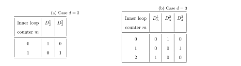
Table 3.1: Illustration of the permutation matrix-based deterministic perturbation sequence construction for two-dimensional and three-dimensional settings.
Hadamard matrices for SPSA
A Hadamard matrix is a square matrix with entries \(\pm 1\) that satisfies \(H\tr H = mI_m\), where \(I_m\) denotes the \(m \times m\) identity matrix. Further, a Hadamard matrix is said to be normalized if all the elements of its first row and column are \(1\). A simple and systematic way of constructing normalized Hadamard matrices of order \(m = 2^k\) is as follows:
For \(k=1\),
\[ H_2 = \left[ \begin{array}{cc} 1 & 1 \\ 1 & -1 \end{array} \right], \]
and for general \(k > 1\),
\[ H_{2^k} = \left[ \begin{array}{cc} H_{2^{k-1}} & H_{2^{k-1}} \\ H_{2^{k-1}} & -H_{2^{k-1}} \end{array} \right]. \]
Let \(P = 2^{\lceil log_2 (d+1) \rceil}\), where, as mentioned before, \(d\) is the parameter dimension. This implies \(P \geq d + 1\). Now construct a normalized Hadamard matrix \(H_P\) of order \(P\) using the above procedure. Let \(h(1),\ldots,h(d)\) be any \(d\) columns other than the first column of \(H_P\). The first column is not considered because all elements in the first column are \(1\), while all the other columns have an equal number of \(+1\) and \(-1\) elements. The latter property aids in cancellation of some of the bias terms. Now form a new matrix \(\widetilde{H}_P\) of order \(P \times d\) with \(h(1),\ldots,h(d)\) as its columns. Let \(\widetilde{\triangle}(k), k=1,\ldots,P\) denote the rows of \(\widetilde{H}_P\). The perturbation sequence \(\{\triangle(m)\}\) is now generated by cycling through the rows of \(\widetilde{H}_P\), i.e.,
\[ \triangle(n) = \widetilde{\triangle}(n \bmod P + 1), \forall n \geq 0. \]
Remark 3.1.
Under assumptions similar to those used in Proposition 3.1, it can be shown that the gradient estimate formed using either permutation matrices for RDSA or Hadamard matrices for SPSA satisfies the following inequality:
\[ \norm{ \EE{\widehat\nabla f(\theta)} \!-\! \nabla f(\theta) } \le C_1\delta^2, \textrm { and } \EE{\norm{ \widehat\nabla f(\theta) - \EE{\widehat\nabla f(\theta)} }^2} \le \frac{C_2}{\delta^2}. \]
3.3.3 Gaussian smoothing
In this section, we analyze the estimation error of a special case of the unified estimate with Gaussian perturbations, using the technique from (Nesterov and Spokoiny 2017).
Let \(y^+= f\left(\theta+\delta \Delta\right)+\xi^{+}\) and \(y=f\left(\theta\right)+\xi^-\), where \(\Delta\) is a \(d\)-dimensional Gaussian vector composed of standard normal r.v.s., i.e., \(\Delta \sim N \left( 0 , I _ { d } \right)\), and \(\xi^+, \xi^-\) are noise factors. Then, the “Gaussian smoothing” gradient estimate is formed as follows:
\[ \begin{align*} \widehat \nabla f(\theta) = \Delta \left[\frac{y^{+} - y}{\delta}\right], \tag{3.15} \end{align*} \]
where \(\Delta\) is a \(d\)-dimensional Gaussian vector composed of standard normal r.v.s., i.e., \(\Delta \sim N \left( 0 , I _ { d } \right)\).
Proposition 3.4.
Assume A3.2, A3.3 and that \(f\) is \(L\)-smooth (see 3.1). The estimate defined in (3.15) satisfies
\[ \begin{align*} \norm{ \EE{\widehat\nabla f(\theta)} - \nabla f(\theta) } &\le C_1\delta, \textrm{ and } \tag{3.16} \\ \EE{\norm{ \widehat\nabla f(\theta) - \EE{\widehat\nabla f(\theta)} }^2} &\le \frac{C_2}{\delta^2}, \tag{3.17} \end{align*} \]
for some constants \(C_1, C_2 > 0\).
Proof.
For any \(\theta\in \R^d\), define
\[ \begin{align*} f_\delta(\theta) &= \frac{1}{(2\pi)^{\frac{d}{2}}}\int_{-\infty}^{\infty} f(\theta+\delta u) \exp\left(-\frac{\l u \r^2}{2}\right)du \\ &= \frac{1}{(2\pi)^{\frac{d}{2}} \delta^d}\int_{-\infty}^{\infty} f(y) \exp\left(-\frac{\l y-\theta \r^2}{2 \delta^2}\right)dy. \end{align*} \]
The function \(f_\delta\) denotes the smoothed version of the objective \(f\), and is obtained by a convolution of \(f\) with Gaussian density. Notice that
\[ \begin{align*} \nabla f_\delta(\theta) &= \frac{1}{(2\pi)^{\frac{d}{2}} \delta^{d+2}}\int_{-\infty}^{\infty} f(y) \exp\left(-\frac{\l y-\theta \r^2}{2 \delta^2}\right) (y-\theta)dy \\ &= \frac{1}{(2\pi)^{\frac{d}{2}}\delta}\int_{-\infty}^{\infty} f(\theta+\delta u) \exp\left(-\frac{\l u \r^2}{2}\right)u\, du \tag{Letting $\delta u=y-\theta$} \\ &= \frac{1}{(2\pi)^{\frac{d}{2}}}\int_{-\infty}^{\infty} \left(\frac{f(\theta+\delta u)-f(\theta)}{\delta}\right)\, \exp\left(-\frac{\l u \r^2}{2}\right)u\, du, \tag{3.18} \end{align*} \]
where the final equality follows by using \(\int_{-\infty}^{\infty} \exp\left(-\frac{\l u \r^2}{2}\right)u\, du=0\). Also,
\[ \begin{align*} \nabla f_\delta(\theta) &= \frac{1}{(2\pi)^{\frac{d}{2}}}\int_{-\infty}^{\infty} \frac{f(\theta)-f(\theta-\delta u)}{\delta}\, \exp\left(-\frac{\l u \r^2}{2}\right)u\, du. \tag{3.19} \end{align*} \]
Using (3.18) and (3.19), we obtain
\[ \begin{align*} \nabla f_\delta(\theta) &= \frac{1}{(2\pi)^{\frac{d}{2}}}\int_{-\infty}^{\infty} \frac{f(\theta+\delta u)-f(\theta-\delta u)}{2\delta}\, \exp\left(-\frac{\l u \r^2}{2}\right)u\, du. \end{align*} \]
Notice that
\[ \begin{align*} &\frac{1}{(2\pi)^{\frac{d}{2}}}\int_{-\infty}^{\infty} \langle\nabla f(\theta),u\rangle\, \exp\left(-\frac{\l u \r^2}{2}\right)u\, du \\ &=\sum_{i=1}^d \nabla_i f(\theta) \frac{1}{(2\pi)^{\frac{d}{2}}}\int_{-\infty}^{\infty} u_i \, \exp\left(-\frac{\l u \r^2 }{2}\right)u\, du \\ &=\sum_{i=1}^d \nabla_i f(\theta) \frac{1}{(2\pi)^{\frac{d}{2}}}\int_{-\infty}^{\infty} \left(u_1 u_i, \ldots,u_{i-1}u_i, u_i^2, u_{i+1} u_i,\ldots, u_i u_d\right) \, \\ &\qquad\qquad\qquad\qquad\qquad\times \exp\left(-\frac{\l u \r^2}{2}\right) du \\ &=\sum_{i=1}^d \nabla_i f(\theta) \frac{1}{(2\pi)^{\frac{d}{2}}} \int_{-\infty}^{\infty} u_i^2\, \exp\left(-\frac{\l u \r^2}{2}\right) du \\ &=\sum_{i=1}^d \nabla_i f(\theta) \frac{1}{(2\pi)^{\frac{d}{2}}} \left(\prod_{j\ne i}\int_{-\infty}^{\infty} \exp\left(-\frac{u_j^2 }{2}\right)\, du_j\right) \int_{-\infty}^{\infty} u_i^2\, \exp\left(-\frac{u_j^2 }{2}\right)\, du_i \\ &= \nabla f(\theta), \tag{3.20} \end{align*} \]
where the penultimate equality uses \(\int_{-\infty}^{\infty} u_i\,u_j \exp\left(-\frac{\l u \r^2}{2}\right)\, du=0\) for \(i\ne j\), which holds owing to the symmetry of the Gaussian distribution. Using (3.20), we obtain
\[ \begin{align*} &\l \nabla f_\delta(\theta) - \nabla f(\theta)\r \\ &\le \frac{1}{(2\pi)^{\frac{d}{2}}\delta}\int_{-\infty}^{\infty} |f(\theta+\delta u)-f(\theta)- \delta \langle\nabla f(\theta)),u\rangle| \, \l u\r \exp\left(-\frac{\l u \r^2}{2}\right) \, du \\ & \le \frac{1}{(2\pi)^{\frac{d}{2}}} \frac{\delta L}{2} \int_{-\infty}^{\infty}\l u\r^3 \exp\left(-\frac{\l u \r^2}{2}\right) \, du \\ &\le \frac{\delta L (d+3)^{\frac{3}{2}}}{2}, \tag{3.21} \end{align*} \]
where the penultimate inequality follows by using the following inequality
\[ |f(y)-f(\theta)- \langle\nabla f(\theta)),y-\theta\rangle| \le \frac{1}{2} L \l \theta-y\r^2, \]
whereas the last inequality is a straightforward moment calculation for a multivariate Gaussian, cf. (Nesterov and Spokoiny 2017 Lemma 1).
The claim in (3.16) concerning the bias of the Gaussian smoothing estimator now follows by combining (3.21) with A3.2.
The claim in (3.17) follows in a similar manner as in the proof of Proposition 3.1.
\(\square\)
We collect a few useful facts about Gaussian smoothing in the following lemma. These facts are extracted from the proof of Proposition 3.4 above.
Lemma 3.1.
Suppose \(f\) is \(L\)-smooth. Let \(f_{\delta}(\theta)\) denote the smoothed functional of \(f\), which is defined as follows: For any \(\theta\in \R^d\),
\[ \begin{align*} f_\delta(\theta) &= \frac{1}{(2\pi)^{\frac{d}{2}}}\int_{-\infty}^{\infty} f(\theta+\delta \Delta) \exp\left(-\frac{\l \Delta \r^2}{2}\right)d\Delta, \end{align*} \]
where \(\Delta\) denotes a standard Gaussian vector.
The gradient of the \(f_\delta(\cdot)\) is given by
\[ \begin{align*} \nabla f_\delta(\theta) &= \frac{1}{(2\pi)^{\frac{d}{2}}}\int_{-\infty}^{\infty} \frac{f(\theta+\delta \Delta)-f(\theta-\delta \Delta)}{2\delta}\, \exp\left(-\frac{\l \Delta \r^2}{2}\right)\Delta\, d\Delta. \end{align*} \]
Further, the smoothed functional \(f_\delta\) is \(L\)-smooth and satisfies
\[ \begin{align*} &\l \nabla f_\delta(\theta) - \nabla f(\theta)\r\le \frac{\delta L (d+3)^{\frac{3}{2}}}{2}. \end{align*} \]
3.3.4 Common random numbers
Consider the classic simulation optimization setting, where the objective is \(f(\theta) = \E(F(\theta,\psi))\), with \(\psi\) denoting the noise element, and \(F(\cdot,\cdot)\) the sample performance. Notice that the observation noise is \(\xi=F(\theta,\psi) - f(\theta)\), and one usually assumes that \(\xi\) is zero-mean, and i.i.d. when one obtains multiple function measurements.
In this section, we consider a special case where \(\psi\) can be kept fixed across function measurements. For instance, one could obtain function measurements \(F(\theta_1,\psi)\) and \(F(\theta_2,\psi)\). More precisely,
\[ f(\theta) = \int F(\theta,\psi) P_{\psi}(d\psi)\,, \tag{3.22} \]
where \(\psi\in \R\) is chosen by the algorithm. To reiterate, the algorithm can call the zeroth-order oracle by selecting both the input parameter \(\theta\) and noise element \(\psi\). In simulation optimization problems, where the function measurements are obtained from a computer simulation, and the source of randomness is common random numbers, one has the luxury of controlling the noise by initializing the seed. Thus, setting the same seed for two different input parameters would amount to having the same set of random numbers across simulations.
In this specialized setting, we now construct a two-point gradient estimate with the same noise element in both function measurements. Let \(y^+= F(\theta+\delta U, \psi)\), and \(y^- = F(\theta- \delta U, \psi)\). Using these function values, we form the gradient estimate as follows:
\[ \begin{align*} \widehat\nabla f(\theta) = \left(\frac{ y^+ - y^-}{2\delta}\right) V. \tag{3.23} \end{align*} \]
We shall establish now that the additional ‘common random noise’ structure allows the algorithm to reduce the variance of the gradient estimates, under the following additional smoothness assumption:
Assumption A3.4.
The function \(F\) has a \(L\)-Lipschitz continuous gradient a.s. for any \(\psi\), i.e.,
\[ \l \nabla F(x,\psi) - \nabla F(y,\psi)\r \le L \l x-y\r \textrm{ a.s.} \]
Proposition 3.5.
Assume A3.1, A3.3, A3.4, and also that the function \(f\) is convex. Then the gradient estimate defined in (3.23) satisfies the following bounds for any given \(\theta\):
\[ \begin{align*} \norm{ \EE{\widehat\nabla f(\theta)} \!-\! \nabla f(\theta) } \le C_1\delta, \textrm { and } \tag{3.24} \\ \EE{\norm{ \widehat\nabla f(\theta) - \EE{\widehat\nabla f(\theta)} }^2} \le C_2 + C_3\delta^2. \tag{3.25} \end{align*} \]
Proof.
As in the proof of Proposition 3.2, for any convex function \(h\) with an \(L\)-Lipschitz gradient, for any \(\delta>0\), we have
\[ \begin{align*} \frac{\<\nabla h(\theta), \delta u\>}{2\delta} \le \frac{h(\theta + \delta u) - h(\theta)}{2\delta} \le& \frac{\<\nabla h(\theta), \delta u\> + (L / 2) \norm{\delta u}^2}{2\delta}. \end{align*} \]
Using similar inequalities for \(h(\theta-\delta u)\), we obtain
\[ \begin{align*} \<\nabla h(\theta), u\> - \frac{L \delta \norm{ u}^2}{2} \le \frac{h(\theta + \delta u) - h(\theta-\delta u)}{2\delta} \le& \<\nabla h(\theta), u\> + \frac{L \delta \norm{ u}^2}{2}. \end{align*} \]
Letting \(\phi(\theta,\delta,u):=\frac1{\delta}\left(\frac{h(\theta + \delta u) - h(\theta-\delta u)}{2\delta} - \<\nabla h(\theta), u\>\right)\), we get
\[ \begin{align*} \left|\phi(\theta,\delta,u) \right| \le& \dfrac{L}{2} \norm{u}^2\,. \end{align*} \]
Using \(\EE{V U^\top}=I\), we obtain
\[ \begin{align*} \E\left[V\, \left(\frac{h(\theta+\delta U) -h(\theta-\delta U)}{2\delta}\right)\right]=& \E\left[ V U^\top\nabla h(\theta) + \delta\phi(\theta,\delta,U) V \right] \\ = & \nabla h(\theta) + \delta \widehat\phi(\theta,\delta), \end{align*} \]
where \(\widehat\phi(\theta,\delta)\) satisfies \(\norm{\widehat\phi(\theta,\delta)} \le \, \dfrac{L}{2}\E[ \norm{V} \norm{U}^2]\).
Applying the above expression to \(F(\cdot, \psi)\) and using (3.23), we have
\[ \E\left[\widehat\nabla f(\theta)\right] = \nabla F(\theta,\psi) + \delta \widehat\phi(\theta,\delta) \textrm{ a.s.}, \]
where \(\widehat\phi(\theta,\delta)\) satisfies \(\norm{\widehat\phi(\theta,\delta)} \le \, \dfrac{L}{2}\E[ \norm{V} \norm{U}^2]\).
A3.4 together with dominated convergence theorem leads to
\(E[\nabla F(\theta,\psi)] = \nabla f(\theta)\). Using this fact, we obtain
\[ \begin{align*} &\norm{\E\left[\widehat\nabla f(\theta)\right] - \nabla f(\theta)} \\ &= \norm{\E\left[V\, \left(\frac{f(\theta+\delta U) -f(\theta-\delta U)}{2\delta}\right)-V U^\top\nabla f(\theta) \right]} \\ &\le \, \delta \norm{\E[ V \phi(\theta,\delta, U)]} \\ &\le \,\frac{\delta L}{2} \E[ \norm{V} \norm{U}^2], \end{align*} \]
and the claim for the bias follows by setting \(C_1= \frac{L}{2} \E[ \norm{V} \norm{U}^2]\).
We now bound \(\EE{ \norm{\widehat\nabla f(\theta)}^2}\) as follows:
\[ \begin{align*} \E \norm{\widehat\nabla f(\theta)}^2 & = \mathbb{E}\norm{V\left(\delta \phi(\theta,\delta, U)+ U^\top\nabla f(\theta) \right)}^2 \\ &\le \E\left[ \left( \norm{ V U \tr \nabla f(\theta)} + \frac{\delta L}{2} \norm{V} \norm{U}^2 \right)^2\right] \\ & \le 2 \E\left[ \norm{ V U \tr \nabla f(\theta)}^2\right] + \frac{\delta^2 L^2}{2}\E\left[ \norm{V}^2 \norm{U}^4 \right], \end{align*} \]
and the claim for the variance follows by setting
\(C_2 = 2 B_1^2 + \frac{ L^2}{2}\E\left[ \norm{V}^2 \norm{U}^4 \right]\) with \(B_1 = \sup_{\theta} \norm{\nabla f(\theta)}\).
\(\square\)
3.3.5 Gradient estimation with truncated Cauchy distribution
One can also use the truncated Cauchy distribution as the smoothing density in smoothed functional algorithms as shown and analyzed recently in (Mondal, Prashanth, and Bhatnagar 2024). We first describe the truncated Cauchy distribution below.
Definition 3.2.
A random variable \(u\) is said to follow the truncated (to the \(\delta\)-sphere) Cauchy distribution with mean vector zero and covariance matrix \(\Sigma = \delta^2\mathbb{I}_{d\times d}\) if \(u\) has the following PDF:
\[ h_\delta(u)=\frac{\Gamma(\frac{d+1}{2})}{\pi^{\frac{d+1}{2}}c_1\delta^d (1+\frac{\lVert u \rVert^2}{\delta^2})^{\frac{d+1}{2}}} \:\:\ \mbox{ for }\: \lVert u \rVert \leq \delta, \tag{3.26} \]
with \(h_\delta(u)=0\) for \(\|u\|>\delta\). In the above, \(c_1>0\) is a normalizing constant.
We define the smoothed version \(g_\delta:\mathbb{R}^d\to\mathbb{R}\) of the given objective function \(f:\mathbb{R}^d\to\mathbb{R}\) as follows:
\[ \begin{align*} g_\delta(\theta)&\triangleq\E_{h_\delta(u)} [f(\theta+u)], \tag{3.27} \end{align*} \]
where \(h_\delta(\theta)\) is the aforementioned smoothing kernel. One may also define another smoothed function \(f_\delta:\R^d\to \R\) based on difference of objectives as follows:
\[ \begin{split} f_\delta(\theta)&=\E_{h_\delta(u)} (f(\theta+ u)-f(\vartheta))\\&=\E_{h_\delta(\theta-u)}[f(u)-f(\theta-u)]. \end{split} \tag{3.28} \]
The following result provides expressions for the gradient of the smoothed functions \(g_\delta\) and \(f_\delta\), respectively. These expressions can be seen to help derive the one-measurement and two-measurement forms for the gradient estimators. We however mention that only the two-measurement form of the gradient estimator in (3.30) below has been studied in (Mondal, Prashanth, and Bhatnagar 2024) as it provides lower bias than the one-measurement form. The reader is referred to (Mondal, Prashanth, and Bhatnagar 2024) for a proof of Proposition 3.6.
Proposition 3.6.
We have
\[ \begin{align*} \nabla g_\delta(\theta) &=\frac{1}{\delta} \mathbb{E}_{u} \left[f(\theta+\delta u) \frac{(d+1)u}{(1+\lVert u \rVert^2)}\right], \tag{3.29} \\ \nabla f_\delta(\theta) &= \frac{1}{\delta} \E_{u} \left[(f(\theta+\delta u)-f(\theta)) \frac{(d+1)u}{(1+\lVert u \rVert^2)}\right]. \tag{3.30} \end{align*} \]
A two-sample gradient estimate \(G(\theta,\xi^+,\xi,u,\delta)\) of \(\nabla f(\theta)\) is formed as follows:
\[ \begin{align*} &G(\theta,\xi^+,\xi,u,\delta) \\ &= \bigg(\frac{F(\theta+\delta u,\xi^+)-F(\theta,\xi)}{\delta}\bigg) \frac{(d+1)u}{(1+\lVert u \rVert^2)}, \tag{3.31} \end{align*} \]
where \(\xi^+\) and \(\xi\) are independent, zero-mean noise random vectors constituting measurement noise in the two function measurements. The function measurements themselves are represented using the function \(F(\cdot)\). Further, the perturbation random variable \(u\sim h_\delta\), the truncated Cauchy PDF.
Assumption A3.5.
The function \(f\) is three-times continuously differentiable with \(\lVert \nabla f(\theta) \rVert\leq B <\infty\) and \(\lVert \nabla_{i_1,i_2,i_3}^3 f(\theta)\rVert\leq B_1\) for all \(\theta\in \R^d\) and for all \(i_1,i_2,i_3=1,\ldots,d\).
Lemma 3.2 (Bias Lemma).
Under Assumption A3.5, we have a.s.
\[ \begin{align*} \E[G(\theta,\xi^+,\xi,u,\delta)|\theta, u]= c_2\nabla f(\theta)+\delta w, \tag{3.32} \end{align*} \]
where \(c_2 = \E_u\left[\frac{(d+1)(u^1)^2}{1+\lVert u\rVert^2}\right]>0\), with \(u^1\) denoting the first component of the random vector \(u\), and \(w = \E\bigg[\bigg(\frac{ u^T\nabla^2 f(\Bar{\theta}^+) u}{2}\bigg)\frac{(d+1)u}{1+\lVert u \rVert^2}|\theta,u\bigg]\) with \(\Bar{\theta}^+\) being a suitable point on the line segment joining \(\theta\) and
\(\theta+\delta u\).
Remark 3.2.
Note here that the bias lemma in this case has a different form than corresponding results in other cases such as the one-sided Gaussian SF, cf. Proposition 3.4. In particular the conditional expectation of \(G(\theta,\xi^+,\xi,u,\delta)\) given \(\theta,u\) has \(O(\delta)\) bias though in comparison with \(c_2\nabla f(\theta)\) instead of \(\nabla f(\theta)\) with \(c_2>0\) as the multiplying factor. We explain in Remark 4.1 about the impact on convergence of the resulting scheme due to this additional factor.
3.3.6 Generalized simultaneous perturbation method
A recently proposed approach in the class of random difference methods is Generalized SPSA (Shalabh Bhatnagar and Prashanth 2023; Pachal, Bhatnagar, and Prashanth 2023). The idea is to use a multi-variate Taylor’s expansion of the objective function at a perturbed parameter and thereafter terminate the expansion after a certain number of terms. The larger the number of terms used in the expansion, smaller is the bias. Thus, the approach allows one to construct finite difference estimators of \(\nabla f(\theta)\) for any given order of the bias. Chapter VII.1a of (Asmussen and Glynn 2007) explores this idea in the context of scalar functions \(f:\mathbb{R}\rightarrow\mathbb{R}\). For the case of vector-valued parameters and for functions \(f:\mathbb{R}^d\rightarrow\mathbb{R}\), this idea has been presented in (Shalabh Bhatnagar and Prashanth 2023; Pachal, Bhatnagar, and Prashanth 2023).
Let \({\displaystyle {\cal D}^\beta f(\theta) = \frac{\partial^{|\beta|}f(\theta)}{\partial\theta_1^{\beta_1}\cdots \partial\theta_d^{\beta_d}}}\) with \(|\beta|=\beta_1+\cdots+\beta_d\) and \(\theta^\beta=\theta_1^{\beta_1}\cdots\theta_d^{\beta_d}\). Further, \(\beta! =\beta_1!\beta_2!\cdots\beta_d!\). The multi-variate Taylor’s expansion has the following form:
\[ f(\theta+\delta\Delta) = \sum_{|\beta|=0}^{\infty} \frac{{\cal D}^\beta f(\theta)}{\beta!}(\delta\Delta)^\beta = \sum_{|\beta|=0}^{\infty} \left(\frac{(\delta\Delta{\cal D})^\beta}{\beta!}\right)f(\theta)=\exp(\delta\Delta{\cal D})f(\theta), \tag{3.33} \]
assuming \(f\) is infinitely many times continuously differentiable. Let \(\tau_{\delta\Delta}f(\theta) \equiv f(\theta+\delta\Delta)\), with \(\tau_{\delta\Delta} = \exp(\delta\Delta{\cal D})\) as the associated shift operator. Thus,
\[ {\cal D} = \frac{1}{\delta\Delta}\log(\tau_{\delta\Delta}), \]
where, \({\displaystyle \frac{1}{\delta\Delta} \stackrel{\triangle}{=} \left(\frac{1}{\delta\Delta_1},\ldots,\frac{1}{\delta\Delta_d}\right)^T. }\) An expansion of the \(\log\) function gives
\[ {\cal D} = \frac{1}{\delta\Delta} \sum_{j=1}^{\infty}\frac{(\tau_{\delta\Delta} - {\cal I})^j}{j}(-1)^{j+1}, \]
where \({\cal I}\) denotes the identity operator and moreover, \(\tau_{\delta\Delta}^k = \tau_{k\delta\Delta}\). The generalized gradient operator can then be viewed as follows: Let \({\cal D} = ({\cal D}_i, i=1,\ldots,d)^T\), where for \(i=1,\ldots,d\),
\[ {\cal D}_i = \frac{1}{\delta\Delta_i} \sum_{j=1}^{\infty}\frac{(\tau_{\delta\Delta} - {\cal I})^j}{j}(-1)^{j+1}. \tag{3.34} \]
From the above, one can obtain an estimator of order \(k\) by taking just the sum of the first \(k\) terms above. This will then require that the function \(f\) be only \(k\) times continuously differentiable and not infinite times continuously differentiable as in the beginning of this section.
Two-measurements (unbalanced) SPSA
The two-measurements version of SPSA here when using the GSPSA estimator (3.34) will correspond to just taking the first term in the summation above. Then, we will get
\[ {\cal D}^1_if(\theta) \stackrel{\triangle}{=} \left(\frac{\tau_{\delta\Delta}-{\cal I}}{\delta\Delta_i} \right) f(\theta) = \frac{f(\theta+\delta\Delta)-f(\theta)}{\delta\Delta_i}, \]
where \({\cal D}^1 = ({\cal D}^1_i, i=1,\ldots,d)^T\) denotes the first order approximation operator. When acting on \(f(\theta)\), it gives the one-sided (unbalanced) version of SPSA, see (Chen, Duncan, and Pasik-Duncan 1999; S. Bhatnagar, Prasad, and Prashanth 2013). Observe that a Taylor’s expansion of \(f(\theta+\delta\Delta)\) around \(\theta\) gives
\[ {\cal D}^1_if(\theta)=\frac{f(\theta+\delta\Delta)-f(\theta)}{\delta\Delta_i} = \frac{\Delta^T\nabla f(\theta)}{\Delta_i} + O(\delta). \tag{3.35} \]
Three-measurements SPSA
This estimator is obtained from (3.34) by truncating the series at \(j=2\).
\[ \begin{align*} {\cal D}^2_if(\theta) &\stackrel{\triangle}{=} \left[ \left(\frac{\tau_{\delta\Delta}-{\cal I}}{\delta\Delta_i}\right) - \frac{(\tau_{\delta\Delta}-{\cal I})^2}{2\delta\Delta_i}\right]f(\theta) \\ &= \left[\left(\frac{\tau_{\delta\Delta}-{\cal I}}{\delta\Delta_i}\right) - \left( \frac{\tau_{2\delta\Delta}+{\cal I} -2\tau_{\delta\Delta}}{2\delta\Delta_i} \right)\right]f(\theta) \\ &= \left(\frac{f(\theta+\delta\Delta)-f(\theta)}{\delta\Delta_i}\right) \\ & \quad- \left(\frac{f(\theta+2\delta\Delta) + f(\theta) - 2f(\theta+\delta\Delta)}{2\delta\Delta_i} \right) \\ &= \left(\frac{4f(\theta+\delta\Delta)-3f(\theta)-f(\theta+2\delta\Delta)}{2\delta\Delta_i}\right). \end{align*} \]
As before, \({\cal D}^2\) indicates the second order approximation operator. This is a new gradient SPSA estimator that has previously not been proposed. Through suitable Taylor’s expansions, one obtains
\[ {\cal D}^2_if(\theta) = \frac{\Delta^T \nabla f(\theta)}{\Delta_i} + O(\delta^2). \tag{3.36} \]
The first term in the expansion in (3.36) is the same as the first term in (3.35). However, the second term in (3.36) is \(O(\delta^2)\) as opposed to \(O(\delta)\) in (3.35).
Four-measurements SPSA
This estimator is obtained from (3.34) by truncating the series at \(j=3\).
\[ \begin{align*} &{\cal D}^3_if(\theta) \\ &= \left[ \left(\frac{\tau_{\delta\Delta}-{\cal I}}{\delta\Delta_i}\right) - \frac{(\tau_{\delta\Delta}-{\cal I})^2}{2\delta\Delta_i} + \frac{(\tau_{\delta\Delta}-{\cal I})^3}{3\delta\Delta_i} \right]f(\theta) \\ &= \Bigg[\left(\frac{\tau_{\delta\Delta}-{\cal I}}{\delta\Delta_i}\right) - \left( \frac{\tau_{2\delta\Delta}+{\cal I} -2\tau_{\delta\Delta}}{2\delta\Delta_i} \right) \\ &\qquad+ \left(\frac{\tau_{3\delta\Delta} -3\tau_{2\delta\Delta} + 3\tau_{\delta\Delta} -{\cal I}}{3\delta\Delta_i} \right)\Bigg]f(\theta) \\ &= \frac{2f(\theta+3\delta\Delta) - 9 f(\theta+2\delta\Delta)+ 18f(\theta+\delta\Delta) -11f(\theta)}{6\delta\Delta_i}. \end{align*} \]
Note that this estimator requires four function measurements at the parameter values \(\theta\), \(\theta+\delta\Delta\), \(\theta+2\delta\Delta\) and \(\theta+3\delta\Delta\), respectively. The RHS above is obtained upon simplification and Taylor’s expansions as before give us in this case
\[ {\cal D}^3_if(\theta) = \frac{\Delta^T \nabla f(\theta)}{\Delta_i} + O(\delta^3). \tag{3.37} \]
The zeroth order as well as second and third order terms turn out to be zero due to cancellations of the various terms in the expansions resulting in (3.37).
Generalized \((k+1)\)-measurements SPSA
Proceeding in a similar manner, one can obtain the \(k\)th order estimator by truncating the series in (3.34) at the \(k\)th term in the summation. Thus, one has in this (general) case
\[ \begin{align*} {\cal D}^k_i &= \frac{1}{\delta\Delta_i} \sum_{j=1}^{k}\frac{(\tau_{\delta\Delta} - {\cal I})^j}{j}(-1)^{j+1} = \frac{1}{\delta\Delta_i} \sum_{l=0}^{k} \frac{(-1)^{1-l} (\tau_{\delta\Delta})^l}{l!} C_l, \end{align*} \]
where \(C_l=\frac{1}{l}\prod\limits_{j=0}^{l-1} (k-j)\). Then,
\[ \begin{align*} {\cal D}^k_if(\theta) & = \left[\frac{1}{\delta\Delta_i} \sum_{l=0}^{k} \frac{(-1)^{1-l} C_l\tau_{l\delta\Delta}}{l!}\right] f(\theta) \\ &= \frac{1}{\delta\Delta_i} \sum_{l=0}^{k} \frac{(-1)^{1-l} C_l f(\theta+l\delta\Delta)}{l!}. \end{align*} \]
This gradient estimator requires \((k+1)\) function measurements at the parameter values \(\theta+l\delta\Delta\), \(l=0,1,\ldots,k\). It has been shown in (Shalabh Bhatnagar and Prashanth 2023; Pachal, Bhatnagar, and Prashanth 2023) that the order \(k\) generalized SPSA algorithm satisfies
\[ {\cal D}^k_if(\theta) = \frac{\Delta^T \nabla f(\theta)}{\Delta_i} + O(\delta^k). \tag{3.38} \]
Remark 3.3.
Several remarks are in order.
As the Taylor’s expansions of the various higher order generalized SPSA algorithms demonstrate, generalized SPSA of order \(k\) has a bias of order \(O(\delta^k)\). Thus, an advantage with this class of algorithms is that given an accuracy level \(O(\delta^k)\), one can find a gradient estimator within this class that provides this level of accuracy. Such guarantees are not available in the classes of estimators seen previously.
Note that here, one need not restrict oneself to only generalized SPSA estimators but in fact, the same can be done for smoothed functional and RDSA based perturbations, see (Pachal, Bhatnagar, and Prashanth 2023).
Finally, note that the estimators presented above are not balanced like two-simulation SPSA. In (Pachal, Bhatnagar, and Prashanth 2023)[Section IV], balanced estimators are also derived by noting that
\[ \tau_{\delta\Delta}f(\theta) - \tau_{-\delta\Delta}f(\theta) = f(\theta+\delta\Delta)-f(\theta-\delta\Delta). \]
A similar calculation as before shows that
\[ \tau_{\delta\Delta}-\tau_{\delta\Delta} = \exp(\delta\Delta\mathcal{D})-\exp(-\delta\Delta\mathcal{D}) = 2\sinh{2\delta\mathcal{D}}. \]
Thus,
\[ \mathcal{D} = \frac{1}{\delta\Delta}\sinh^{-1}{\left(\frac{\tau_{\delta\Delta}-\tau_{-\delta\Delta}}{2}\right)}. \]
Balanced estimators requiring even number of function measurements are then presented by terminating the infinite series of the \(\sinh^{-1}(\cdot)\) function after varying number of steps.
We refer the reader to (Pachal, Bhatnagar, and Prashanth 2023) for detailed proofs of non-asymptotic and asymptotic convergence of the algorithms derived using the above gradient estimators.
3.4 Summary
| Property \(\bm{ \rightarrow}\) Gradient estimate \(\bm{\downarrow}\) Two-point estimate (3.6), $f | Bias | Variance |
| Two-point estimate ([3.6](#book-eq-grad-unified-83d424 \(f\) convex+smooth One-point estimate (3.12), $f | )) | \(C_1 \delta\) \(\dfrac{C_2}{\delta^2}\) |
| One-point estimate ([3.12](#book-eq-grad-one-point-82e \(f\) convex+smooth Gaussian smoothing (3.15), $f | e55)) | \(C_1 \delta^2\) \(\dfrac{C_2}{\delta^2}\) |
| Gaussian smoothing with \(L\)-smooth \(F\), \(C_1 \delta\) $C_2 + C_3ommon random noise | elta^2$ |
3.5 Bibliographic remarks
The idea of simultaneous perturbation dates back to (Katkovnik and Kulchitsky 1972), where the authors proposed the smoothed functional scheme for gradient estimation. A closely related estimation scheme is RDSA, proposed by (Kushner and Clark 1978), where the random perturbation are chosen uniformly on the surface of a \(d\)-dimensional sphere. This idea is equivalent to using \(d\)-dimensional standard Gaussian vector for the random perturbations — a choice studied in (Polyak and Tsybakov 1990; Dippon 2003; Shalabh Bhatnagar and Borkar 2003; S. Bhatnagar 2007; Nesterov and Spokoiny 2017). The asymptotic convergence of a zeroth-order algorithm with Gaussian smoothing where the gradient is estimated using a single measurement \(y^+ = f(\theta+\delta\Delta)+\xi^+\) alone is shown in (Shalabh Bhatnagar and Borkar 2003). The same with a balanced estimator with two measurements \(y^+ = f(\theta+\delta\Delta)+\xi^+\) and \(y^- = f(\theta-\delta\Delta)+\xi^-\) is shown in (S. Bhatnagar 2007). The latter reference also proposes one and two measurement Newton algorithms where both the gradient and Hessian are estimated using \(y^+\) and \(y^-\) respectively. In (Rubinstein 1981), conditions on perturbation distributions needed to construct zeroth-order gradient estimators have been presented. It is also shown that the uniform, Cauchy and Gaussian distributions satisfy these properties. Simultaneous perturbation gradient search algorithms with \(q\)-Gaussian smoothed functionals have been proposed in (Ghoshdastidar, Dukkipati, and Bhatnagar 2014) for a wide range of the \(q\)-value parameter, for which the aforementioned distributions namely uniform, Cauchy and Gaussian emerge as special cases for certain values of \(q\). It is shown that Variants of RDSA, employing uniform and asymmetric Bernoulli distributed random perturbations, have been proposed recently in (Prashanth et al. 2017). SPSA, proposed by (Spall 1992), is a very popular simultaneous perturbation method, which also exhibits the lowest asymptotic mean-square error (cf. (Chin 1997; Prashanth et al. 2017)). Deterministic perturbation variants of SPSA have been proposed and analyzed in (Shalabh Bhatnagar et al. 2003), while the corresponding deterministic variation for RDSA has been proposed recently in (Prashanth et al. 2020). A comprehensive text-book reference on simultaneous perturbation methods is (S. Bhatnagar, Prasad, and Prashanth 2013). The latter reference contains a rigorous treatment of SPSA/SF methods, and includes both first as well as second-order schemes.
We now briefly survey other recent work on stochastic optimization. In (Berahas et al. 2022), the authors assume the measurement noise is bounded a.s. and analyze simultaneous perturbation-based gradient estimators under this condition. In particular, they establish bounds on the bias and variance of the gradient estimators and also conduct detailed numerical experiments comparing the performance of finite difference-based estimators with those employing simultaneous perturbation on a synthetic setup. In (Gasnikov et al. 2022), zeroth-order stochastic optimization algorithms for non-smooth convex optimization problems are presented with perturbations distributed uniform on the surface of a unit sphere. Bounds on the number of iterations needed as well as the complexity of the estimator are provided. In (Kozak et al. 2023; Rando et al. 2023, 2024), one-sided zeroth-order gradient estimation algorithms for both convex objectives as well as non-convex objectives, involving perturbation matrices with orthogonal random directions are presented. At each iterate, a random matrix \(\mathbb{P}\) of size \(d\times l\) is obtained with in general, fewer columns than rows and satisfying the conditions (i) \(\mathbb{P}\tr \mathbb{P} = (d/l) \mathbb{I}\) and (ii) \(\E[\mathbb{P}\mathbb{P}\tr]=\mathbb{I}\) (the identity matrix). A total of \(l\) zeroth order gradient estimates are then obtained and summed with each column of the \(\mathbb{P}\) matrix. This is then used in the gradient update procedure. Various cases such as coordinate descent, spherical smoothing etc., are then considered, and rate bounds on the algorithm in both non-convex and convex cases are obtained. Almost sure convergence of the iterates in the convex case is also shown in (Rando et al. 2024).
Another recent work along these lines in (Wang and Feng 2024). Measurement noise is not considered in the system observations and the only noise that is present is in the gradient search directions. The convergence rates of such algorithms for Lojasiewicz functions which are generalizations of the Polyak-Lojasiewicz (PL) functions are obtained. Assuming existence of an almost sure limit point of the parameter sequence \(\theta_n, n\geq 0\), the rate of convergence of \(\{f(\theta_n)\}\) and \(\{\theta_n\}\) is obtained. For a class of smooth as well as convex and non-smooth Lojasiewicz functions, the convergence is shown to be faster than standard zeroth-order gradient search. The work of (Kornowski and Shamir 2024) provides a zeroth-order stochastic optimization scheme that produces the complexity of obtaining a \((\delta,\epsilon)\)-stationary point of a possibly non-smooth and non-convex Lipschitz objective. Their algorithm incorporates a two-measurement gradient estimator using a common random noise sequence and with perturbations that are distributed uniform on the unit sphere. The proposed algorithm requires \(O(d\delta^{-1}\epsilon^{-3})\) function evaluations which the authors argue is the best complexity obtained so far.
There is also work on algorithms that provide better bounds due to reduced variance in the iterates. In (Duchi, Bartlett, and Wainwright 2012), a stochastic optimization algorithm for a smoothed convex function that works with sub-differentials is presented that is however not a zeroth-order stochastic optimization scheme. The authors consider sample average of the estimates and show that the same has a better (finite-time) convergence rate due to the resulting lower variance in the iterates with extra averaging. Zeroth-order stochastic gradient search algorithms with variance reduction have been presented in (Ji et al. 2019). In (Huang, Tao, and Chen 2020), a class of Franke-Wolfe methods using zeroth-order stochastic gradient estimation approaches involving an accelerated scheme with reduced variance are presented. Their approach shows improved function query complexity for finding an approximate stationary point.
For the sake of simplicity, we have chosen to hide the constants through a \(O(\delta^3)\) term. The latter constants can be made precise, as in Proposition 3.1 below.↩︎
Here and in what follows, \(\xi^+\) and \(\xi^-\) are real valued r.v.s and this notation is not be confused with positive and negative parts of a measurable function (Royden and Fitzpatrick 2010).↩︎