2 Stochastic approximation
In this chapter, we provide an introduction to stochastic approximation algorithms, and outline a few popular applications such as mean estimation, gradient-type algorithms, fixed-point iterations, and quantile estimation. We provide the main asymptotic convergence results under two approaches, namely ODE and differential inclusions. The former approach is applicable to Lipschitz continuous objective functions, which allows viewing a linearly-interpolated stochastic approximation algorithm’s sample path as approximating the trajectory of an ODE. Using this ‘dynamical systems’ viewpoint, we list the assumptions that ensure almost sure convergence of stochastic approximation iterates to the equilibria of the underlying ODE. The approach of recursive inclusions is useful for handling objective functions with discontinuities. As in the ODE case, the stochastic approximation algorithm’s interpolated trajectory is seen as an approximation to that of the recursive inclusion, leading to an almost sure convergence result. In the context of this book, when the perturbation constant \(\delta\), which features in the simultaneous perturbation-based gradient estimator presented above, is taken to zero, the stochastic gradient algorithm’s behavior can be analyzed using ODEs, while treatment of a constant \(\delta\) requires one to consider a differential inclusions-based analysis.
2.1 Introduction
The basic stochastic approximation recursion is of the following form:
\[ \theta_{n+1} = \theta_n + a(n)(h(\theta_n) + M_{n+1}), \tag{2.1} \]
where \(\theta_n \in \mathbb{R}^d\), \(n\geq 0\), is the stochastic sequence of iterates that are updated according to (2.1), \(h:\mathbb{R}^d\rightarrow \mathbb{R}^d\) is a point-to-point map, \(M_{n+1}, n\geq 0\) is the associated noise sequence, and the multipliers \(a(n), n\geq 0\) form a sequence of positive step sizes or learning rates.
Under certain conditions on the aforementioned quantities that we shall discuss in this chapter, one can show that the recursion (2.1) almost surely tracks asymptotically the limit sets of the ODE (2.2) in a manner that will be made precise later.
\[ \dot{\theta}(t) = h(\theta(t)). \tag{2.2} \]
We shall also consider here generalizations of the scheme (2.1) via stochastic recursive inclusions as well as recursions with an additional Markov noise component. Stochastic recursive inclusions are algorithms as in (2.1) except that the function \(h(\theta)\) is in general a set instead of a point for any given \(\theta\). Such a scheme in general will have the following form:
\[ \theta_{n+1} = \theta_n + a(n)(y_n + M_{n+1}), \tag{2.3} \]
where \(M_n,n\geq 0\) is the noise sequence as before and \(y_n\in h(\theta_n)\), where it will be now assumed that \(h:\mathbb{R}^d\rightarrow\mathbb{R}^d\) is a set-valued map. Under some assumptions, such recursions will also be seen to almost surely track asymptotically the underlying differential inclusion
\[ \dot{\theta}(t)\in h(\theta(t)). \tag{2.4} \]
The reader is referred to Appendix A for an introduction to ODEs and differential inclusions.
2.2 Applications
We begin with a few well-known applications of stochastic approximation. These include minimizing a function given noisy function measurements, which forms the core content of this book, as well as estimation of various quantities, e.g., mean, fixed-point, quantile, from noisy observations.
2.2.1 Mean estimation
Consider a random variable (r.v.) \(\X\) with mean \(\mu\) and variance \(\sigma^2\). Suppose we are given independent and identically distributed (i.i.d.) samples \(X_1, \dots, X_n\) from the distribution of \(\X\). Let \(\theta_n=\frac{1}{n} \sum_{k=1}^n X_k\) be the sample mean computed using these \(n\) samples. We now derive an iterative scheme for updating the sample mean.
\[ \begin{align*} \theta_{n+1} &= \dfrac{1}{n+1} \sum_{k=1}^{n+1} X_k = \dfrac{n}{n+1} \left(\dfrac{1}{n} \sum_{k=1}^n X_k \right) + \dfrac{1}{n+1} X_{n+1} \\ &= \dfrac{n}{n+1} \theta_n + \dfrac{1}{n+1} X_{n+1} \\ \theta_{n+1} &= \theta_n + \dfrac{1}{n+1} \left(X_{n+1} - \theta_n\right). \tag{2.5} \end{align*} \]
The update rule above is a stochastic approximation scheme with step size \(a(n) = \frac{1}{n+1}\), \(n\geq 0\).
By the strong law of large numbers, one obtains
\[ \begin{align*} \theta_n &\rightarrow \mu \text{\; a.s. as \;} n \rightarrow \infty. \end{align*} \]
One may instead use a more general step size sequence \(a(n),n\geq 0\) and write the update rule (2.5) as
\[ \begin{align*} \theta_{n+1} &= \theta_n + a(n) \left(X_{n+1} - \theta_n\right) \\ &= \theta_n + a(n) \left[\left(\mu-\theta_n\right) + \left(X_{n+1}-\mu\right)\right] \end{align*} \]
Letting \(M_{n+1}=X_{n+1}-\mu\), it is easy to see that \(M_{n},n\geq 0\) is a martingale difference sequence1 satisfying \(\E M_n^2 < \infty\).
From an application of the Kushner-Clark lemma, to be presented later, it can again be shown that \(\theta_n \rightarrow \mu\) almost surely as \(n \rightarrow \infty\) and this happens for general step sizes that satisfy the following conditions (see Theorem 2.4(i)):
\[ \sum_n a(n)=\infty \text{ and } \sum_n a(n)^2<\infty. \tag{2.6} \]
Clearly \(a(n)=1/(n+1)\) is a special case of the above. This means that the above result using the strong law of large numbers continues to hold with more general step sizes. The Kushner-Clark lemma is the main tool to infer asymptotic convergence of stochastic approximation algorithms. We shall present a precise statement and a proof of this result in Section 2.3.
2.2.2 Stochastic gradient algorithm using unbiased gradient information
Consider the following problem: Find
\[ \theta^* \in \arg\min_{\theta} f(\theta), \tag{2.7} \]
where \(f\) is a smooth function (see Appendix D for background material on smoothness).
A stochastic gradient algorithm for solving (2.7) would update as follows:
\[ \begin{align*} \theta_{n+1} = \theta_n - a(n) \widehat\nabla f(\theta_n). \tag{2.8} \end{align*} \]
In the above, \(\widehat\nabla f(\theta_n)\) is an estimate of the gradient \({\nabla} f(\theta_n)\), and \(\{a(n)\}\) are (pre-determined) step sizes satisfying standard stochastic approximation conditions (see (2.6) above).
Here we shall assume unbiased gradient information is available, i.e., \(\E\left[ \widehat\nabla f(\theta_n) \mid \theta_n\right] = \nabla f(\theta_n)\). In this case, the algorithm in (2.8) becomes an instance of the seminal stochastic approximation scheme proposed by Robbins and Monro in 1951. The latter algorithm was proposed to find the zeroes of a function, and in the case of (2.8), the function of interest is \(\nabla f\). If the gradient estimates \(\widehat\nabla f(\theta_n)\) have bounded variance, then the algorithm in (2.8) can be shown to converge to the stationary points of \(f\). We make this claim precise later in Section 4.1.
We now describe a popular optimization setting, where unbiased gradient information is available. Consider the following problem that is ubiquitous in machine learning applications involving training over a given dataset of \(m\) samples, say \(\{(x_i,y_i), i=1,\ldots,m\}\):
\[ \min_\theta f(\theta) = \frac{1}{m} \sum_{i = 1}^m f_i(\theta). \tag{2.9} \]
In the above, \(f_i\) denotes the loss associated with sample \(i\). A simple example is the square-loss in a linear regression problem, where \(f_i(\theta)= (y_i-\theta\tr x_i)^2\). It is common to assume that the loss functions \(f_i, \forall i\) are smooth, and \(f\) is convex or strongly convex.
A batch gradient descent algorithm would solve the problem above using the following update iteration:
\[ \theta_{n+1} = \theta_n - a(n)\left(\frac{1}{m}\sum_{i = 1}^m \nabla f_i(\theta_n)\right). \tag{2.10} \]
The above algorithm is a noise-less algorithm, and for large \(m\), it is computationally expensive. In ML parlance, \(m\) is the number of training examples.
A computationally efficient alternative is stochastic gradient descent, popularly known as SGD. This algorithm involves picking a training sample uniformly at random, i.e., a r.v. \(i_n\) with the following distribution:
\[ i_n = \begin{cases} 1 & \text{w.p. } \frac{1}{m}\\ . & \\ . & \\ m & \text{w.p. } \frac{1}{m}. \end{cases} \]
SGD would then update the iterate as follows:
\[ \theta_{n+1} = \theta_n - a(n) \nabla f_{i_n}(\theta_n). \tag{2.11} \]
Rewriting the above update rule, we obtain
\[ \begin{align*} \theta_{n+1} &= \theta_n -\alpha_n\left(\frac{1}{m}\sum_{i = 1}^m \nabla f_i(\theta_n)\right) -\alpha_n\left(\nabla f_{i_n}(\theta_n) - \frac{1}{m}\sum_{i=1}^m \nabla f_i(\theta_n)\right) \\ &= \theta_n - \alpha_n\left(\frac{1}{m}\sum_{i =1}^m \nabla f_i(\theta_n) + w_{n+1}\right), \end{align*} \]
where {\(w_{n+1} = \nabla f_{i_n}(\theta_n) - \frac{1}{m}\sum_{i =1}^m \nabla f_i(\theta_n)\)} is a martingale difference sequence because \(\E[w_{n+1}|\theta_1, \ldots \theta_n] = 0\).
Several applications involving learning and optimization involve martingale difference noise terms, and the convergence of the stochastic approximation algorithm is tied to whether the effect of underlying noise (martingale difference) can be ignored in the long run. For an introduction to martingales, the reader is referred to Appendix B.
2.2.3 Stochastic gradient algorithm using a zeroth-order oracle
In a zeroth-order setting, the gradient information is not directly available, and instead, the optimization algorithm has oracle access to noise-corrupted function measurements, as illustrated in the figure below.

The stochastic gradient algorithm updates as follows:
\[ \begin{align*} \theta_{n+1} = \theta_n - a(n) \widehat\nabla f(\theta_n), \tag{2.12} \end{align*} \]
where \(\widehat\nabla f(\theta_n)\) is formed from the function measurements. Two such gradient estimators, using two function measurements, were presented earlier in (1.6) and (1.9), respectively. Such estimates are not unbiased, but feature a parameter that can reduce the bias at the cost of variance. In the next chapter, we present the simultaneous perturbation trick that generalizes the example in (1.9).
Under suitable assumptions, \(\theta_n,n\geq 0\), governed by (2.12) can be shown to converge almost surely to the set \(\bar{H}=\{ x \mid \nabla f(\theta) = 0 \}\). We provide this result later in Section 4.1.
2.2.4 Stochastic fixed point iterations
Consider a function \(f:\R^d\rightarrow\R^d\) that satisfies
\[ \begin{align*} \norm{f(x)-f(y)} \le \alpha \norm{x-y}, \tag{2.13} \end{align*} \]
for any \(x,y\in \R^d\). Here \(\alpha \in (0,1)\), and \(\norm{\cdot}\) is the \(\ell_2\)-norm associated with \(\R^d\). Such an \(f\) is called a contraction map. Since the underlying space is complete, by the Banach fixed point theorem, there exists a unique fixed point \(\theta^*\) of the function \(f\).
A first attempt at finding such a fixed point is via the following iterative scheme: start with some \(\theta_0 \in \R^d\) and update as
\[ \theta_{n+1} = f (\theta_n). \]
A smoothened variation to this update rule is given by
\[ \begin{align*} \theta_{n+1} = (1-a(n)) \theta_n + a(n) f(\theta_n), \end{align*} \]
where \(a(n)\) is the step size. Note that if \(\theta_n \rightarrow \theta^*\) and \(f\) is continuous at \(\theta^*\), then \(f(\theta^*) = \theta^*\).
So far we have assumed that \(f\) is perfectly observable for any given input parameter. However, in many learning scenarios, e.g., reinforcement learning, this isn’t the case. In particular, consider the setting where \(f\) is not precisely known, but we have black box access to \(f\), as illustrated in Figure 2.1. The simplest noise model would correspond to i.i.d., e.g., \(\mathcal{N}(0,1)\), while a martingale difference noise structure is more general.
For this setting, a stochastic fixed point iteration would update as follows:
\[ \begin{align*} \theta_{n+1} = (1-a(n)) \theta_n + a(n) (f(\theta_n) + \xi_{n+1}), \tag{2.14} \end{align*} \]
where as described above, a simple setting is where \(\{\xi_n\}\) is an i.i.d. sequence with \(\E\left[\xi_n\right] = 0\), and \(\E\l\xi_n\r^2 < \infty\), for all \(n\). Now, it is desirable to have \(\theta_n \rightarrow \theta^*\) almost surely as \(n \rightarrow \infty\). From the convergence analysis of stochastic approximation algorithms, to be presented later, we shall see that \(\theta_n \rightarrow \theta^*\) if (i) \(f\) is a contraction, see (2.13); (ii) step sizes satisfy standard stochastic approximation conditions, see (2.6); and (iii) noise \(\xi_n\) is a martingale difference sequence that has bounded variance, or satisfies a linear growth condition (see Assumption A2.8 below).
Remark 2.1.
The stochastic fixed point iteration algorithm discussed above would not necessarily converge if the modulus of contraction \(\alpha=1\) in (2.13). In this case, a fixed point is not even guaranteed to exist, e.g., consider \(f(\theta)=\theta+1\). Alternatively, more than one fixed point may exist (e.g., \(f(\theta)=\theta\)), or only one fixed point exists (e.g. \(f(\theta)=-\theta\)). Under an additional assumption that at least one fixed point exists, the stochastic fixed point iteration (2.14) is guaranteed to converge almost surely to a sample path dependent fixed point solution.
Stochastic fixed point iterations are ubiquitous in the context of reinforcement learning. In particular, the well-known TD-learning and Q-learning algorithms are stochastic fixed-point iterations. The reader is referred to (D. P. Bertsekas 2012; Sutton and Barto 2018; D. P. Bertsekas and Tsitsiklis 1996) for a detailed introduction to these algorithms.
2.2.5 Linear stochastic approximation
Consider the following stochastic approximation algorithm:
\[ \theta_{n+1} = \theta_n + a(n)\left( A_{n+1} \theta_n + b_{n+1} \right), \]
where the step size \(a(n)\) satisfies \(\sum_n a(n) = \infty\), and \(\sum_n a(n)^2 < \infty\). Further, \(A_n\) and \(b_n\) are matrices and vectors that satisfy
\[ \E\left[A_{n+1} \mid \theta_1,\ldots,\theta_n\right] = A, E\left[b_{n+1} \mid \theta_1,\ldots,\theta_n\right] = b, \]
where \(A\) is a negative-definite matrix. Moreover, \(\E\left[\norm{ (A_{n} - A)}^2\right] \le C_1\) and \(\E\left[ \norm{b_n - b}^2 \right] \le C_2\). In this setting, applying the Kushner-Clark lemma (to be presented later), it can be shown that
\[ \theta_n \rightarrow \theta^* \textrm{ a.s. as } n \rightarrow \infty, \]
where the limit \(\theta^*\) satisfies \(A\theta^*+b=0\).
A prominent LSA algorithm is TD-learning with linear function approximation, see (J. N. Tsitsiklis and Van Roy 1997). Other examples include solving a linear regression problem using a stochastic gradient algorithm (Prashanth, Korda, and Munos 2021; Mou et al. 2020), and linear approximations to non-learning SA recursions (S. Chen et al. 2020).
2.2.6 Quantile estimation
Consider the following problem, which is a variant of mean estimation. For a continuous random variable (r.v.) \(X\) with cumulative distribution function \(F\) and for a given \(\alpha \in (0,1)\), define
\[ q_\alpha(X) = F^{-1}(\alpha). \]
Notice that \(q_\alpha(X)\) is the median of the distribution of \(X\) when \(\alpha=0.5\). Let \(\{X_n\}_{n\ge 1}\) be a independent sequence of r.v.s with common distribution \(F\). Notice that \(F(q_\alpha(X))=\E[\indic{X\le q_\alpha(X)}]=\alpha\). A stochastic approximation algorithm for estimating \(q_\alpha(X)\) for a pre-specified \(\alpha\) can be arrived at as follows: Let \(q_n\) denote an estimate of \(q_\alpha(X)\) after observing samples \(X_1,\ldots,X_n\). On observing \(X_{n+1}\), \(q_n\) is updated as follows:
\[ \begin{align*} q_{n+1} = q_n + a(n) \left( \indic{X_{n+1} \le q_n} - \alpha \right), \tag{2.15} \end{align*} \]
where \(\indic{\cdot}\) denotes the indicator function, i.e., \(\indic{A}=1\) if \(A\) happens and \(0\) otherwise.
Notice that the update is iterative, i.e., given an estimate \(q_n\) at time instant \(n\) and a new sample \(X_{n+1}\), the algorithm should perform an incremental update using \(q_n, X_{n+1}\) to arrive at \(q_{n+1}\).
Consider the following alternative observation model: At time instant \(n\), the stochastic approximation algorithm picks a threshold, say \(T\), and the environment returns a Boolean that indicates whether \(X_{n+1} < T\) or not. Quantile estimation in this threshold-based model would follow the same iterative scheme as (2.15). To see this, let
\[ Y_{n+1}=\begin{cases} 1 & \textrm{ if } X_{n+1} \le q_n\\ 0 & \textrm{ else}. \end{cases}. \]
Then, the update rule in (2.15) is equivalent to
\[ \begin{align*} q_{n+1} = q_n + a(n) \left( Y_{n+1} - \alpha \right). \tag{2.16} \end{align*} \]
Using a variant of Kushner Clark lemma, to be presented later, it is possible to establish almost sure convergence of \(q_n\) to \(q_\alpha(X)\).
In finance literature, a risk measure closely related to quantiles is ‘Value at Risk (VaR)’. For any random variable \(X\), we define the VaR at level \(\alpha\in\left(0,1\right)\) as
\[ \text{VaR}_{\alpha}(X) =\inf\left\{\xi \mbox{ }|\mbox{ }\mathbb{P}\left(X\leq \xi\right)\geq\alpha\right\}. \]
If the distribution of \(X\) is continuous, then VaR is the lowest solution to \(\mathbb{P}\left(X\leq \xi\right)=\alpha.\) VaR as a risk measure has several drawbacks, which precludes using standard stochastic optimization methods. This motivated the definition of coherent risk measures in (Artzner et al. 1999). A risk measure is coherent if it is convex, monotone, positive homogeneous and translation equi-variant. Conditional Value at Risk (CVaR) is a popular risk measure defined by
\[ \begin{align*} \text{CVaR}_{\alpha}(X) =\inf_{\xi} \left\lbrace \xi + \frac{1}{(1-\alpha)}\E\left( X -\xi\right)_+ \right\rbrace, \tag{2.17} \end{align*} \]
where \((a)_+=\max(a,0)\) denotes the positive part of a real number \(a\). For a continuous random variable \(X\), it can be shown that
\[ \text{CVaR}_{\alpha}(X):=\mathbb{E}\left[X | X \geq \text{VaR}_{\alpha}(X)\right]. \]
Unlike VaR, the above is a coherent risk measure.
A well-known result from (Rockafellar and Uryasev 2000) is that both VaR and CVaR can be obtained from the solution of a certain convex optimization problem and we recall this result next.
Theorem 2.1.
For any random variable \(X\) and a \(\alpha\in (0,1)\), let
\[ \begin{align*} v(\xi,X):=\xi + \frac{1}{1-\alpha}(X-\xi)_{+} \text{ and } V(\xi)=\E\left[v(\xi,X)\right]. \tag{2.18} \end{align*} \]
Then, \(\textnormal{VaR}_{\alpha}(X)=\left(\arg\min V:= {\left\{\xi \in \mathbb{R}\ | \ V'(\xi)=0 \right\}}\right)\), where \(V'\) is the derivative of \(V\) w.r.t. \(\xi\). Further, \(\textnormal{CVaR}_{\alpha}(X)=V(\textnormal{VaR}_{\alpha}(X))\).
From the above, it is clear that in order to estimate VaR/CVaR, one needs to find a \(\xi\) that satisfies \(V'(\xi)=0\). Stochastic approximation (SA) is a natural tool to use in this situation. Recall that SA is used to solve the equation \(h(\theta) = 0\) when analytical form of \(h\) is not known. However, noisy measurements \(h(\theta_n) + \xi_n\) can be obtained, where \(\theta_n, n \ge 0\) are the input parameters and \(\xi_n, n \ge 0\) are zero-mean random variables, that are not necessarily i.i.d.
Using the stochastic approximation principle and the result in Theorem 2.1, we have the following scheme to estimate the VaR/CVaR simultaneously from the samples \(\{X_1,\ldots,X_n\}\):
\[ \begin{align*} \text{VaR: } & q_{n+1}= q_{n}-a(n)(1-\frac{1}{1-\alpha}\indic{X_{n+1}\geq q_n}), \tag{2.19} \\ \text{CVaR: } & \psi_{n+1}=\psi_{n}-\frac{1}{n+1}\left(\psi_{n} - v(q_{n},X_{n+1})\right). \tag{2.20} \end{align*} \]
In the above, (2.19) can be seen as a gradient descent rule, while (2.20) can be seen as a plain averaging update. Since CVaR estimate depends on the VaR estimate, whereas the converse is not true, the update recursions (2.19)–(2.20) exhibit a one-way coupling, which implies the \(1/(n+1)\) step size in (2.20) can be replaced by \(a(n)\) for the sake of analysis.
An interesting question is whether the stochastic gradient-based estimation scheme in (2.19) converges faster than the root-finding estimation scheme in (2.15).
2.3 Convergence analysis using the ODE approach
So far, we have provided an introduction to stochastic approximation, and outlined a few popular applications. We now cover preliminary results on the convergence of stochastic approximation algorithms using the limit sets of the associated ordinary differential equation (ODE). In the next section, we provide convergence results with stochastic recursive inclusions, i.e., those algorithms that involve set-valued maps.
Consider now the following recursion:
\[ \theta_{n+1} = \theta_n + a(n) (h(\theta_n) + \beta_n+ \eta_n). \tag{2.21} \]
Definition 2.1.
We denote by \(L(\{\theta_n,n\geq0\})\) the limit set of the sequence \(\theta_n,n\geq 0\) obtained from (2.21). In other words, it is the set of all limit points of the sequence \(\{\theta_n\}\) obtained from (2.21). Thus, consider all such subsequences \(\{n_m\}\) of \(\{n\}\) with \(n_m\rightarrow \infty\) for which \(\theta_{n_m}\rightarrow \check{\theta}\) for some \(\check{\theta}\in \mathbb{R}^d\). The collection of all these points \(\check{\theta}\) obtained as limits of such subsequences \(\{\theta_{n_m}\}\) of \(\{\theta_n\}\) is defined as \(L(\{\theta_n,n\geq0\})\). Note also that \(L(\{\theta_n,n\geq 0\})\) is a sample-path dependent set that can vary in general from one sample path to another.
Consider the following ODE associated with (2.21):
\[ \dot{\theta}(t) = h(\theta(t)). \tag{2.22} \]
This is the same ODE as (2.2). Define a sequence \(\{t(n),n\geq 0\}\) of time points as follows:
\[ t(0)=0, \mbox{ } t(n) = \sum_{k=0}^{n-1} a(k), n\geq 1. \tag{2.23} \]
We now state the main result for the convergence of (2.21), see Theorem 1.2 of (Benaïm 1996)), under the assumptions below.
Assumption A2.1.
\(h:\mathbb{R}^d\rightarrow\mathbb{R}^d\) is a Lipschitz continuous function with Lipschitz constant \(L>0\).
Assumption A2.2.
\(\lim_{n\rightarrow\infty} \beta_n=0\) w.p.1.
Assumption A2.3.
The step sizes satisfy \(a(n)>0\), \(\forall n\), \(a(n)\rightarrow 0\) as \(n\rightarrow\infty\) and \(\sum_n a(n)=\infty\).
Assumption A2.4.
For each \(T>0\), \(\epsilon>0\),
\[ \lim_{n\rightarrow\infty} P \left( \sup_{j\geq n}\max_{t\leq T} \parallel \sum_{i=m(jT)}^{m(jT+t)-1} a(i)\eta_i \parallel\geq \epsilon \right) =0 \mbox{ w.p.}1, \]
where
\[ m(t) = \left\{\begin{array}{cc} \max\{n|t(n)\leq t\}, & t\geq 0,\\ 0 & t <0. \end{array}\right. \]
Assumption A2.5.
\(\sup_n \left\| \theta_n\right\| <\infty\) w.p.1.
Assumption A2.6.
There exists a locally asymptotically stable attractor \(\theta^*\in \mathbb{R}^d\) of the ODE (2.22) with domain of attraction \(\check{\Omega}\subset \mathbb{R}^d\).
We now discuss these assumptions. Assumption A2.1 ensures that the ODE (2.22) is well-posed. Assumption A2.2 ensures that the bias \(\beta_n\) vanishes asymptotically. We shall discuss Assumption A2.3 and Assumption A2.4 in detail below. Assumption A2.6 is satisfied for most gradient systems. This assumption can however be easily relaxed to the case where the attractor is a compact connected set of points instead of being ‘isolated’. Theorem 2.2 however takes the form of Theorem 2.3 (a more general result) when one does not have an attractor in the underlying system.
The stability requirement in A2.5, while hard to ensure directly, is common to the analysis of stochastic approximation algorithms. A commonly used procedure to ensure stability is to employ a projection operator onto a large enough compact and convex constraint set that keeps the iterate sequence \(\{\theta_n\}\) bounded. One then uses the following update rule in place of (4.7):
\[ \begin{align*} \theta_{n+1} = \Pi\left(\theta_n + a(n) (h(\theta_n) + \beta_n+ \eta_n)\right), \tag{2.24} \end{align*} \]
where \(\Pi\) is a projection operator that keeps the iterates bounded within a compact and convex set, say \(\Theta \subset \R^d\). For instance, a computationally inexpensive projection onto \(\Theta \stackrel{\triangle}{=} \prod_{i=1}^d[\theta_{\min}^i, \theta_{\max}^i]\) can be realized by setting \(\Pi_i(\theta) = \min(\max(\theta_{\min}^i,\theta^i),\theta_{\max}^i),\ i\in \{1 \hdots d\}\). If the projected region \(\Theta\) contains all the attractors of the gradient ODE, then \(\theta_n\) updated according to (2.24) would likely converge to such an attractor, except that the projection set boundary also introduces spurious attractors, see (Kushner and Yin 2003). In the case when some of the attractors lie outside the constraint set, the iterate-sequence \(\theta_n,n\geq 0\), may get stuck at the boundary of \(\Theta\), trying to push forward in the direction of the aforementioned attractors. To avoid the latter situation, one could gradually grow the region of projection as suggested in (H. F. Chen, Guo, and Gao 1987), or perform projection infrequently as in (Dalal et al. 2018). In (V. G. Yaji and Bhatnagar 2019), the iterate sequence is reset to a compact set at increasingly sparse instants (in case it goes out of that set) if the mean field has a globally attracting set. Such a scheme is shown to remain both stable and convergent in (V. G. Yaji and Bhatnagar 2019) with the number of resets remaining finite.
The focus of this book is gradient estimation in a zeroth-order setting, and for the analysis, we assume that the iterates are stable. As discussed above, one could employ a projection operator, to workaround the stability issue, see Section 2.4 for further details. Also, independent of projection, certain verifiable sufficient conditions for stability of stochastic approximations in the literature, cf. (Borkar and Meyn 2000) and (Abounadi, Bertsekas, and Borkar 2002) for two such conditions, and (A. Ramaswamy and Bhatnagar 2016) and (A. Ramaswamy and Bhatnagar 2021) for similar conditions in the context of set-valued stochastic approximation.
Motivation for step size assumptions:
One can reason about the need for the step size conditions using a simpler noise setting as follows: Suppose \(\beta_n = 0, \forall n\) and \(\{\eta_n\}\) is an i.i.d. sequence with mean zero and variance \(\sigma^2\). Then, variance of \(\theta_{n+1}\) is
\[ \begin{align*} \Var(\theta_{n+1}) &= \Var\left[\theta_n + a(n) h(\theta_n) \right] + a(n)^2 Var(\eta_{n+1}) \\ &= \Var\left[\theta_n + a(n) h(\theta_n) \right] + a(n)^2 \sigma^2 \\ &\geq a(n)^2 \sigma^2. \end{align*} \]
If we choose a constant stepsize, i.e., \(a(n) = a \; \forall n\), then, \(Var(\theta_{n+1}) \geq a^2 \sigma^2\). Thus, with a constant step size, \(\theta_n \not\longrightarrow \theta^*\) almost surely, motivating the need for having a diminishing step size that vanishes asymptotically. However, such a step size cannot go down too fast, since
\[ \begin{align*} \theta_{m+1} &= \theta_m + a(m) (h(\theta_m) + \eta_{m+1} ), \\ \l\theta_m - \theta_0\r &\leq \sum_{\tau = 0}^{m-1} a(\tau) |h(\theta_\tau) + \eta_{\tau+1}| \end{align*} \]
If \(|h(\theta_\tau) + \eta_{\tau+1}| \leq C_1\) and \(\sum_{\tau=0}^\infty a(\tau) \leq C_2 < \infty\), then \(\l\theta_m - \theta_0\r\) is bounded above. This implies that \(\theta_m\) is forced to be within a ball of radius \(C_1C_2\) around the initial point \(\theta_0\), for all \(m\). This then puts an artificial constraint on \(\{\theta_m\}\) as \(\theta^*\) can always lie outside this ball. Thus, we need \(\sum_\tau a(\tau) = \infty\).
Remark 2.2 (Only Diminishing vs. Square Summable Step-Sizes).
Assumption A2.3 is a condition on the step-size sequence \(\{a(n)\}\) and is weaker than standard Robbins-Monro step-size requirements such as Assumption A2.7 that requires square summability of the step-sizes. However, as Theorems 2.2 and 2.3 suggest, if one makes Assumption A2.3 on the step-size sequence, then one needs to additionally make Assumption A2.4 on the noise sequence \(\{\eta_n\}\). Verifying the latter independently may not be straightforward.
On the other hand, assuming the noise sequence \(\eta_n,n\geq 0\) is a martingale difference satisfying Assumption A2.8, one can prove that Assumption A2.4 holds under Assumption A2.7 and Assumption A2.5. This is indeed shown in Remark 2.4. As mentioned, this will require the step-size sequence to be square summable, not just asymptotically diminishing. Theorem 2.4 is a variant of Theorem 2.3 that is based on Assumptions A2.7–A2.8 in place of Assumptions A2.3–A2.4, respectively, while continuing with the other assumptions.
The original convergence result of Kushner and Clark, see Theorem 2.3.1 of (Kushner and Clark 1978), that establishes convergence of (2.21) is the following:
We briefly present a proof of this result which follows along the lines of Theorem 2.3.1 of (Kushner and Clark 1978). A more generalized result is then provided as Theorem 2.3 which is from (Benaïm 1996) [Theorem 1.2].
Proof.
Recall the stochastic recursion (2.21):
\[ \theta_{n+1} = \theta_n + a(n) (h(\theta_n) + \beta_n+ \eta_n). \]
Let \(\theta^0(t),t\geq 0\), denote a continuous linear interpolation of the \(\theta_n\) iterates obtained as follows: For \(t\in [t(n),t(n+1)]\), \(n\geq 0\),
\[ \theta^0(t) = \frac{t(n+1)-t}{t(n+1)-t(n)} \theta_n + \frac{t-t(n)}{t(n+1)-t(n)} \theta_{n+1}. \]
Similarly, for \(t\) as above, let
\[ \beta^0(t) = \frac{t(n+1)-t}{t(n+1)-t(n)} \left(\sum_{i=0}^{n-1}a(i)\beta_i\right) + \frac{t-t(n)}{t(n+1)-t(n)} \left(\sum_{i=0}^{n}a(i)\beta_i\right), \]
\[ \eta^0(t) = \frac{t(n+1)-t}{t(n+1)-t(n)} \left(\sum_{i=0}^{n-1}a(i)\eta_i\right) + \frac{t-t(n)}{t(n+1)-t(n)} \left(\sum_{i=0}^{n}a(i)\eta_i\right), \]
respectively. We also define a piecewise constant interpolated process \(\bar{\theta}^0(\cdot)\) according to
\[ \bar{\theta}^0(t) = \theta_n, \mbox{ } \theta\in [t(n),t(n+1)). \]
Then the recursion (2.21) can be written in continuous time as
\[ \theta^0(t) = \theta^0(0) +\int_{0}^{t} h(\bar{\theta}^0(\tau))d\tau + \beta^0(t) +\eta^0(t), \mbox{ }t\geq 0. \tag{2.25} \]
From these continuous-time functions, we define a sequence of left-shifted functions \(\theta^n(\cdot),\beta^n(\cdot),\eta^n(\cdot)\) as follows: For \(n\geq 0\),
\[ \theta^n(t) = \left\{ \begin{array}{cc} \theta^0(t+t(n)), & t\geq -t(n)\\ \theta_0, & t\leq -t(n) \end{array}\right. \]
\[ \eta^n(t) = \left\{ \begin{array}{cc} \eta^0(t+t(n))-\eta^0(t(n)), & t\geq -t(n)\\ -\eta^0(t(n)), & t\leq -t(n) \end{array}\right. \]
\[ \beta^n(t) = \left\{ \begin{array}{cc} \beta^0(t+t(n))-\beta^0(t(n)), & t\geq -t(n)\\ -\beta^0(t(n)), & t\leq -t(n) \end{array}\right. \]
respectively.
Before proceeding further, we show that under Assumption A2.3 and Assumption A2.4, \(\eta^0(\cdot)\) is uniformly continuous on \([0,\infty)\) almost surely. Further, for any \(0<T<\infty\),
\[ \lim_{t\rightarrow\infty} \sup_{|s|\leq T} \|\eta^0(t+s)-\eta^0(t)\| = 0 \mbox{ w.p.}1. \]
By Assumption A2.4, given \(\epsilon>0\), there exists \(n_k>0\) such that
\[ P\left(\sup_{j\geq n_k} \max_{t\leq T} \| \sum_{i=m(jT)}^{m(jT+t)-1} a(i)\eta_i\| \geq \epsilon\right) \leq \frac{1}{2^k}. \]
Thus,
\[ \sum_{k} P\left(\sup_{j\geq n_k} \max_{t\leq T} \| \sum_{i=m(jT)}^{m(jT+t)-1} a(i)\eta_i\| \geq \epsilon\right) <\infty. \]
Thus, corresponding to \(\{n_k\}\), we get a sequence of events \(\{E_k\}\) where
\[ E_k = \{\sup_{j\geq n_k} \max_{t\leq T} \| \sum_{i=m(jT)}^{m(jT+t)-1} a(i)\eta_i\| \geq \epsilon\}. \]
By the Borel-Cantelli lemma, \(P(E_k\) infinitely often\()=0\). Thus,
\[ \sup_{\{|s|\leq T, t\geq n_k\}} \|\eta^0(t+s)-\eta^0(t)\| <\epsilon, \]
for all but finite number of \(n_k\) (integers) w.p.1. Since \(\eta^0(\cdot)\) is continuous w.p.1 on \([0,\infty)\), the above implies that \(\eta^0(\cdot)\) is also uniformly continuous w.p.1. Thus, \(\{\eta^n(\cdot)\) is uniformly continuous on \(\mathbb{R}\), bounded on compacts and \(\eta^n(\cdot)\rightarrow 0\) w.p.1 uniformly on compacts in \(\mathbb{R}\). Likewise, from Assumption A2.2, \(\{\beta^n(\cdot)\}\) is uniformly continuous on \(\mathbb{R}\), bounded on compacts and \(\beta^n(\cdot)\rightarrow 0\) w.p.1 uniformly on compacts in \(\mathbb{R}\).
Now, (2.25) can be equivalently written as follows: For \(t\geq 0\),
\[ \theta^n(t) = \theta^n(0) +\int_{0}^{t} h(\bar{\theta}^0(t(n)+\tau))d\tau + \beta^n(t) +\eta^n(t) \]
\[ = \theta^n(0) +\int_{0}^{t} h(\theta^n(\tau))d\tau + \epsilon^n(t)+ \beta^n(t) +\eta^n(t), \tag{2.26} \]
where
\[ \epsilon^n(t) = \int_{0}^{t} h(\bar{\theta}^0(t(n)+\tau))d\tau - \int_{0}^{t} h(\theta^n(\tau))d\tau. \]
Note that by Lipschitz continuity of \(h(\cdot)\) (cf. Assumption A2.1),
\[ \|\epsilon^n(t)\| \leq L\int_{0}^{t}\|\bar{\theta}^0(t(n)+\tau)) - \theta^n(\tau))\|d\tau, \tag{2.27} \]
where \(L>0\) is the Lipschitz constant of the function \(h(\cdot)\). Now, observe that
\[ \theta^n(t) = \theta^0(t+t(n)) = \bar{\theta}^0(t+t(n)) + \int_{0}^{t} h(\bar{\theta}^0(t(n)+\tau))d\tau + \beta^n(t)+\eta^n(t). \]
Thus,
\[ \|\theta^n(t)-\theta^0(t+t(n))\| \leq \int_{0}^{t} \|h(\bar{\theta}^0(t(n)+\tau))\| d\tau + \|\beta^n(t)\| + \|\eta^n(t)\|. \tag{2.28} \]
Now, by Lipschitz continuity of \(h(\cdot)\),
\[ \|h(\bar{\theta}^0(t(n)+\tau))\| - \|h(0)\| \leq \|h(\bar{\theta}^0(t(n)+\tau)) - h(0)\| \]
\[ \leq L\|\bar{\theta}^0(t(n)+\tau)\|. \]
Thus, with \(\check{L}=\max(L,\|h(0)\|)\), we get that
\[ \|h(\bar{\theta}^0(t(n)+\tau))\| \leq \check{L}(1+\|\bar{\theta}^0(t(n)+\tau)\|). \]
Since, outside a set of zero probability, \(\exists \check{M}>0\) such that \(\|\bar{\theta}^0(t(n)+\tau)\| \leq \check{M}\). Thus,
\[ \|h(\bar{\theta}^0(t(n)+\tau))\| \leq \check{K}, \]
where \(\check{K} \stackrel{\triangle}{=} \check{L}(1+\check{M})>0\). Thus, from (2.28), it follows that
\[ \|\theta^n(t)-\theta^0(t+t(n))\| \leq a(n) \check{K} + \|\beta^n(t)\| + \|\eta^n(t)\|. \]
The RHS above \(\rightarrow 0\) as \(n\rightarrow\infty\) uniformly on compact intervals. Substituting the above inequality in (2.27), one obtains
\[ \|\epsilon^n(t)\| \leq La(n)(a(n)\check{K} + \|\beta^n(t)\|+\|\eta^n(t)\|) \rightarrow 0, \]
as \(n\rightarrow\infty\) uniformly on compact intervals. Thus, \((\epsilon^n(t)+\beta^n(t)+\eta^n(t))\rightarrow 0\) as \(n\rightarrow\infty\) uniformly on compact intervals. From Assumption A2.5, \(\{X^n(\cdot)\}\) is bounded and further it is easy to observe that this sequence is equicontinuous. From the Arzela-Ascoli theorem, it then follows that \(\{\Theta^n(\cdot)\}\) is relatively compact. Thus, there exists a convergent subsequence that we continue to call \(\{\theta^n(\cdot)\}\) itself without loss of generality. Let \(\theta(\cdot)\) be the limiting function of this sequence. Then \(\theta(\cdot)\) can be seen to satisfy the limiting ODE (2.22) as
\[ \theta(t) = \theta(0) + \int_{0}^{t} h(\theta(\tau))d\tau, \]
which is the integral form of the ODE (2.22).
Now note that under Assumption A2.6, \(\theta^*\in\mathbb{R}^d\) is an attractor for the ODE (2.22). Let \(\epsilon_1,\epsilon_2>0\) be two scalars with \(\epsilon_1<\epsilon_2\) with \(\epsilon_1\) being small in particular. Then the \(\epsilon_1\) and \(\epsilon_2\) neighborhoods of \(\theta^*\) satisfy \(N_{\epsilon_1}(\theta^*) \subset N_{\epsilon_2}(\theta^*)\) and let \(N_{\epsilon_2}(\theta^*) \subset A\). Since \(\theta_n\in A\) infinitely often, it follows that there exists a subsequence \(\{n_m\}\) of \(\{n\}\) such that \(\theta_{n_m}\in A, \forall n_m\). Consider then the process \(\theta^{n_m}(\cdot)\) which will have a subsequence (also indexed by \(\{n_m\}\) for simplicity) that will converge to a limit \(\hat{\theta}(\cdot)\) that in turn will satisfy the ODE (2.22). Since \(\hat{\theta}(0)\in A\) and \(\theta^*\) is asymptotically stable, \(\hat{\theta}(t)\rightarrow\theta^*\) as \(t\rightarrow\infty\).
Consider again the process \(\theta^{n_m}(\cdot)\) formed from the stochastic iterates. Since \(\theta^{n_m}(\cdot)\rightarrow\hat{\theta}(\cdot)\) uniformly on compacts and \(\hat{\theta}(t) \rightarrow \theta^*\), it follows that there is a subsequence \(\{\theta_{n_{mj}}\}\) of \(\{\theta_{n_m}\}\) that will be contained in \(N_{\epsilon_1}(\theta^*)\). However, we know that \(\{\theta_{n_m}\}\) is entirely contained in \(A\). Suppose then that there is a subsequence \(\{\theta_{n_{mk}}\) of \(\{\theta_{n_m\}}\) that is entirely contained in \(A\backslash N_{\epsilon_2}(\theta^*)\), i.e., \(A\cap N^c_{\epsilon_2}(\theta^*)\). Then \(\{\theta_{n_m}\}\) will move from \(N_{\epsilon_1(\theta^*)}\) to \(A\backslash N_{\epsilon_2}(\theta^*)\) and back infinitely often since there are an infinite number of points in each of these sets. Then there is a sequence of time points \(\tau_1<\bar{\tau}_1<\tau_2<\bar{\tau}_2\cdots\) such that \(\theta^0(\tau_j)\in \partial N_{\epsilon_1}(\theta^*)\) and \(\theta^0(\bar{\tau}_j)\in \partial N_{\epsilon_2}(\theta^*)\), \(\forall j\). Further, \(\theta^0(t) \in \bar{N}_{\epsilon_2}(\theta^*)\backslash N_{\epsilon_1}(\theta^*)\), for \(t \in (\tau_j,\bar{\tau}_j)\) for all \(j\). Consider the \([\tau_j,\bar{\tau}_j]\) portions of the trajectory \(\theta^0(\cdot)\). This sequence will have a convergent subsequence whose limit is say \(\tilde{\theta}(\cdot)\) which again satisfies (2.22). Consider two cases: (i) There is a \(T>0\) such that along a subsequence \(\bar{\tau}_j-\tau_j \rightarrow T\). Then, \(\tilde{\theta}(0) \in \partial N_{\epsilon_1}(\theta^*)\) and \(\tilde{\theta}(T) \in \partial N_{\epsilon_2}(\theta^*)\). This is not possible by asymptotic stability of \(\theta^*\) since \(\epsilon_1>0\) is small. (ii) Let \(r_j-l_j\rightarrow\infty\). Then the set of \(\{[l_j,\infty)\}\) segments of \(\theta^0(\cdot)\) are bounded and equicontinuous. Again by the Arzela-Ascoli theorem, one can obtain a convergent subsequence with limit say \(\check{\theta}(\cdot)\) that again satisfies (2.22). Then \(\check{\theta}(0) \in \partial N_{\epsilon_1}(\theta^*)\) and \(\check{\theta}(t) \in \bar{N}_{\epsilon_2}(\theta^*)\backslash N_{\epsilon_1}(\theta^*)\). This contradicts that \(\theta^*\) is asymptotically stable. The claim follows.
\(\square\)
Remark 2.3.
A more formal argument on the tracking of the iterate sequence to the underlying ODE (2.22) is provided in Chapter 2 of (Borkar 2022). We briefly sketch that argument here for completeness.
Consider \(\{t(n)\}\) as in (2.23) and let \(T>0\) be a given time element and define a sequence of time points \(\{T_n\}\) as follows: Let \(T_0=t(0)=0\). Further, for \(n\geq 1\), let
\[ T_n = \min\{t(m) | t(m)\geq T_{n-1}+T\}, \]
denote a sequence of time points. Let \(\theta^{T_n}(t), t\geq T_n\) denote the solution to the ODE (2.22) with \(\theta^{T_n}(T_n) = \theta^0(T_n)\) as the initial condition of the ODE. It is argued in Lemma 1, Chapter 2, of (Borkar 2022), using an application of the Gronwall’s inequality (see Lemma A.1), that
\[ \lim_{n\rightarrow\infty} \max_{t\in [T_n,T_{n+1}]} \|\theta^0(t)-\theta^{T_n}(t)\| =0, \]
almost surely. In fact, the above holds for any time point \(s\in\mathbb{R}\) (in positive and negative time), not just the time instants \(T_n\) above. Now if the ODE has a globally asymptotically stable attractor \(A\), any trajectory of the ODE (2.22) will eventually converge to it, and so will the interpolated iterates \(\theta^0(t)\), and thereby the iterate sequence \(\theta_n,n\geq 0\). Figure 2.2 illustrates this iterate-tracking process.
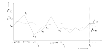
Figure 2.2: The continuously interpolated algorithm’s trajectory \(\theta^0(t)\) represented by the solid line asymptotically tracks the ODE’s trajectory (the dashed-dotted line) \(\theta^{T_n}(t)\) suitably reset to the algorithm’s trajectory after every (regular) time interval approximately \(T\) instants long. On the \(X\)-axis are the instants \(t(0),t(1),\cdots\), with \(t(n)-t(n-1)=a(n)\), \(\forall n\) with \(t(0)=0\). From the step size conditions, it follows that \(t(n)\rightarrow\infty\) as \(n\rightarrow\infty\). This ensures that the algorithm does not converge prematurely.
This result is a generalization of the Kushner and Clark lemma (cf. (Kushner and Clark 1978)) and is stated under the same assumptions as used in the aforementioned result.
We now state some alternative assumptions that in fact we shall use for our analysis.
Assumption A2.7.
\(a(n)>0, \forall n, \text{ } \sum_n a(n)=\infty \text{ and } \sum_n a(n)^2<\infty.\)
Assumption A2.8.
\(\{\eta_n\}\) is a square integrable martingale difference sequence with respect to the filtration \(\{\mathcal{F}_n\}\), with \(\mathcal{F}_n = \sigma(\theta_m, \beta_m, m\leq n, \eta_m, m<n)\), \(n\geq 0\). Further,
\[ \E [\l \eta_{n+1} \r^2 \mid \F_n] \le C_0 (1 + \l \theta_n \r^2), \ n\ge 0. \]
Remark 2.4.
As discussed in Remark 2.2, Assumption A2.7 is stronger than Assumption A2.3. However, Assumptions A2.7 and A2.8, in addition to A2.5 turn out to be sufficient conditions for the verification of Assumption A2.4. This can be seen as follows: Let
\[ \chi_n = \sum_{m=0}^{n-1} a(m) \eta_m, n\geq 1. \]
Then, from Assumption A2.8, it will follow that \((\chi_n,\F_n), n\geq 0\) is a martingale sequence. Moreover,
\[ \begin{align*} &E\left[\sum_n \|\chi_{n+1}-\chi_n\|^2\mid \mathcal{F}_n\right] \\ &= E\left[\sum_n a(n)^2\|\eta_n\|^2\mid \mathcal{F}_n\right] \\ &\leq \sum_n a(n)^2 C_0 \left(1+\|\theta_n\|^2\right) \tag{by Assumption~A2.8} \\ &<\infty \textrm{ a.s. } \tag{ by Assumption~A2.5.} \end{align*} \]
Thus the quadratic variation process associated with the martingale \(\{\chi_n\}\) is almost surely convergent. Hence, by the martingale convergence theorem for square integrable martingales, see Theorem B.7 in Appendix B, \(\{\chi_n\}\) itself is almost surely convergent. Assumption A2.4 will thus follow.
We now present the generalized form of the Kushner-Clark theorem for convergence of algorithms of the form (2.21), where we also consider the case when \(h(\theta)=-\nabla f(\theta)\), for a continuously differentiable function \(f:\mathbb{R}^d\rightarrow\mathbb{R}\). This result is stated under Assumptions A2.1, A2.2, A2.7, A2.5 and A2.8 and will be used for the analysis of our gradient search algorithms. In this case, the recursion (2.21) takes the form
\[ \theta_{n+1} = \theta_n + a(n) (-\nabla f(\theta_n) + \beta_n+ \eta_n), \mbox{ }n\geq 0. \tag{2.29} \]
The ODE associated with (2.29) is the following:
\[ \dot{\theta}(t) = -\nabla f(\theta(t)). \tag{2.30} \]
Theorem 2.4.
The recursion (2.21), under Assumptions A2.1, A2.2, A2.5, A2.7, A2.8, converges almost surely to \(L(\{\theta_n, n\geq 0\})\), see Definition 2.1. Further, \(L(\{\theta_n, n\geq 0\})\) is a connected internally chain recurrent set for the ODE (2.22).
Part (i) continues to hold for the case of (2.29) where \(h(\theta)=-\nabla f(\theta)\) for a continuously differentiable function \(f:\mathbb{R}^d\rightarrow\mathbb{R}\) and with the ODE (2.30) in place of (2.22). Further, \(L(\{\theta_n, n\geq 0\}) \subset H\stackrel{\triangle}{=}\) \(\{\theta \mid \nabla f(\theta) = 0\}\).
Remark 2.5.
As mentioned previously, Theorem 2.4(i) is similar to Theorem 2.3 except that it is obtained under more directly verifiable noise condition in Assumption A2.8 as opposed to AssumptionA2.4 and under step-size Assumption A2.7 in place of Assumption A2.3.
In the case of stochastic gradient recursions as in (2.29), one can claim a stronger result, see Theorem 2.4(ii). In this case, \(H=\{\theta|\nabla f(\theta)=0\}\) denotes the set of all equilibria of the ODE (2.30), for which \(V(\theta)=f(\theta)\) serves as a Lyapunov function since
\[ \begin{align*} \frac{dV(\theta)}{dt} &= \langle \nabla V(\theta),\dot{\theta}\rangle \\ & = \langle \nabla V(\theta), -\nabla V(\theta)\rangle \\ & \leq 0, \mbox{ }\forall \theta\in\mathbb{R}^d. \end{align*} \]
In particular, \({\displaystyle \frac{dV(\theta)}{dt} <0}\), \(\forall \theta\not\in H\) and \({\displaystyle \frac{dV(\theta)}{dt} =0}\) otherwise. Finally, Theorem 2.4(ii) is similar to Corollary 2.1 of (Borkar 2022) even though the latter is stated for the case of a general recursion (not necessarily of the gradient type) but where a Lyapunov function exists for an ODE such as (2.22).
Note also that in the case of (2.29), if \(L(\{\theta_n,n\geq 0\})\) comprises of only isolated limit points, then by Theorem 2.4(ii), these limit points of the algorithm constitute isolated equilibria of the ODE (2.30), and \(\theta_n,n\geq 0\) will converge almost surely to a possibly sample path dependent equilibrium, see Corollary 2.2 of (Borkar 2022).
Remark 2.6.
Stability of stochastic approximation, i.e., Assumption A2.5, is one of the strongest requirements to ensure convergence of the stochastic iterates. Various sets of sufficient conditions to ensure stability of the stochastic iterates can be found in (Kushner and Yin 2003; Borkar and Meyn 2000; Abounadi, Bertsekas, and Borkar 2002; John N. Tsitsiklis 1994) and other references.
2.4 Projected Stochastic Approximation
There are many practical situations where it is difficult to verify sufficient conditions for stability (as in Remark 2.6) of the stochastic recursions. In such scenarios, a popular approach is to enforce stability on the stochastic iterates by selecting a convex and compact set in which the parameter iterates can take values and thereafter projecting the iterates to the aforementioned set whenever the iterates escape from the same. This approach also helps in situations where the parameter takes values only in a pre-specified compact set. Stability of the iterates is then enforced due to the projection.
We review here an important result originally due to Kushner and Clark (cf. Theorem 5.3.1 on pp. 191-196 of (Kushner and Clark 1978)) that shows the convergence of projected stochastic approximations. While the result, as stated in (Kushner and Clark 1978), is more generally applicable, we present its adaptation here that is relevant to the setting that we consider.
Let \(C\subset {\cal R}^d\) be a compact and convex set and \(\Gamma:{\cal R}^d\rightarrow C\) denote a projection operator that projects any \(\theta=(\theta_1,\ldots,\theta_d)^T \in {\cal R}^d\) to its nearest point in \(C\). Thus, if \(\theta\in C\), then \(\Gamma(\theta)\in C\) as well. For instance, if \(C\) is a \(d\)-dimensional rectangle having the form \({\displaystyle C = \prod_{i=1}^{d} [a_{i,\min}, a_{i,\max}]}\), where \(-\infty< a_{i,\min} < a_{i,\max} <\infty\), \(\forall i=1,\ldots,d\), then a convenient way to identify \(\Gamma(\theta)\) is according to \(\Gamma(\theta)=(\Gamma_1(\theta_1),\ldots,\Gamma_N(\theta_d))^T\), where the individual operators \(\Gamma_i:{\cal R}\rightarrow {\cal R}\) are defined by
\[ \Gamma_i(\theta_i) = \min(a_{i,\max}, \max(a_{i,\min},\theta_i)), \mbox{ } i=1,\ldots,d. \]
Let \({\cal C}(C)\) denote the space of all continuous functions from \(C\) to \({\cal R}^d\).
Consider the following \(d\)-dimensional stochastic recursion:
\[ \theta_{n+1} = \Gamma(\theta_{n} + a(n)(h(\theta_n) + \xi_n + \beta_n)), \tag{2.31} \]
under the assumptions listed below.
Consider now the following ODE associated with (2.31):
\[ \dot{\theta}(t) = \bar{\Gamma}(h(\theta(t))). \tag{2.32} \]
Here, \(\bar{\Gamma}: {\cal C}(C)\rightarrow {\cal C}({\cal R}^d)\) is defined according to
\[ \bar{\Gamma}(v(\theta)) = \lim_{\eta\rightarrow 0} \left(\frac{\Gamma(\theta+\eta v(\theta))-\theta}{\eta}\right), \tag{2.33} \]
for any continuous \(v:C\rightarrow {\cal R}^d\). The limit in (2.33) exists and is unique since \(C\) is a convex set. In case \(C\) is not convex, the limit \(\bar{\Gamma}(v(\theta))\) in (2.33) will not be unique in general for all \(\theta\) and so \(\bar{\Gamma}(h(\theta(t)))\) will be a set of points for any \(\theta(t)\), that is not necessarily a singleton, and so instead of the ODE (2.32), one may consider the following differential inclusion:
\[ \dot{\theta}(t) \in \bar{\Gamma}(h(\theta(t))). \tag{2.34} \]
A similar result as below can then be seen to hold in this case. For simplicity, we shall restrict our attention to the case where \(C\) is a compact and convex set.
From the definition of \(\bar{\Gamma}\) in (2.33), note that \(\bar{\Gamma}(v(\theta)) = v(\theta)\) if \(\theta\in C^o\) (the interior of \(C\)). This is because for such a \(\theta\), one can find \(\eta>0\) sufficiently small so that \(\theta+\eta v(\theta) \in C^o\) as well and hence \(\Gamma(\theta+\eta v(\theta)) = \theta+\eta v(\theta)\). On the other hand, if \(\theta\in \partial C\) (the boundary of \(C\)) is such that \(\theta+\eta v(\theta) \not\in C\), for any small \(\eta>0\), then \(\bar{\Gamma}(v(\theta))\) is the projection of \(v(\theta)\) to the tangent space of \(\partial C\) at \(\theta\).
Consider now the assumptions listed below.
Assumption A2.9.
The function \(h:{\cal R}^d\rightarrow {\cal R}^d\) is continuous.
Assumption A2.10.
The step sizes \(a(n),n\geq 0\) satisfy
\[ a(n)>0\ \forall n, \mbox{ } \sum_n a(n)=\infty, \mbox{ } \sum_n a(n)^2 <\infty. \]
Assumption A2.11.
The sequence \(\beta_n,n\geq 0\) is a bounded random sequence with \(\beta_n \rightarrow 0\) almost surely as \(n\rightarrow \infty\).
Assumption A2.12.
\(\{\eta_n\}\) is a square integrable martingale difference sequence with respect to the filtration \(\{\mathcal{F}_n\}\), with \(\mathcal{F}_n = \sigma(\theta_m, \beta_m, m\leq n, \eta_m, m<n)\), \(n\geq 0\). Further,
\[ \E [\l \eta_{n+1} \r^2 \mid \F_n] \le C_0 (1 + \l \theta_n \r^2), \ n\ge 0. \]
Let \(K\subset \mathcal{R}^d\) denote the set of asymptotically stable attractors of (2.32). Then, (Kushner and Clark 1978 Theorem 5.3.1 (pp. 191-196)) essentially says the following:
Remark 2.7.
We wish to point out that the original theorem of Kushner and Clark (cited above) for the case of projected stochastic approximations is stated for the case of an analogous assumption as Assumption A2.4 in place of A2.12 and Assumption A2.3 in place of A2.10. As discussed in Remark 2.4, the noise assumption A2.12 in conjunction with A2.10 (and the fact that now the iterates are uniformly bounded throughout because of the projection), imply A2.4. Moreover, these assumptions are more easily verifiable in most applications.
2.5 Stochastic Recursive Inclusions
In many applications, one encounters set-valued maps \(h(\theta)\), \(\theta\in \mathbb{R}^d\) in place of point-to-point maps \(h(\theta)\), for instance, resulting from dealing with partial observation settings. Let \(h:\mathbb{R}^d \rightarrow \{\mbox{set of subsets of } \mathbb{R}^d\}\). A stochastic recursive inclusion has the following structure:
\[ \theta_{n+1} -\theta_n -a(n) M_{n+1} \in a(n) h(\theta_n), \tag{2.35} \]
where \((M_n,\mathcal{F}_n),n\geq 0\), is a martingale difference sequence. Consider now the associated differential inclusion (DI):
\[ \dot{\theta}(t) \in h(\theta(t)). \tag{2.36} \]
Let \(t(n),n\geq 0\) be a sequence of time points defined as follows: \(t(0)=0\) and for \(n\geq 1\), \({\displaystyle t(n)= \sum_{k=0}^{n-1} a(k)}\). Thus, \(t(n+1)=t(n) + a(n)\). For any \(t\geq 0\), let \(m(t)\stackrel{\triangle}{=} \sup\{k\geq 0\mid t\geq t(k)\}\). Define a continuous time affine interpolated process \(W:[0,\infty)\rightarrow \mathbb{R}^d\) as follows:
\[ W(t(n)+s) = \theta_n + s \left(\frac{\theta_{n+1}-\theta_n}{a(n)}\right), \mbox{ } s\in [0,a(n)]. \]
From the above, \(W(t(n))=\theta_n, \forall n\). Recall Definition A.12 for definition of a perturbed solution to a DI. The following result is from (Benaïm, Hofbauer, and Sorin 2005 Proposition 1.3).
Proposition 2.1.
Assume the following hold:
For all \(T>0\),
\[ \lim_{n\rightarrow\infty}\sup\{\|\sum_{k=n}^{l-1}a(k)M_{k+1} \| \mid k=n+1,\ldots,m(t(n)+T)\}=0. \]
\(\sup_n\|\theta_n\| <\infty\) almost surely.
Then the process \(W(\cdot)\) is a perturbed solution of the DI (2.36).
Consider now the assumptions A2.7-A2.8 with \(\eta_n=M_{n+1}, n\geq 0\) as the martingale difference sequence. Assume also the stability requirement on the iterates (2.35).
Assumption A2.13.
The iterates (2.35) satisfy \(\sup_n\|\theta_n\| <\infty\) almost surely.
Let \({\displaystyle \zeta(n) = \sum_{m=0}^{n-1} a(m)M_{m+1}}\), \(n\geq 1\). Then \((\zeta(n),\mathcal{F}_n),n\geq 1\) can be seen to be a martingale sequence. From Assumptions A2.8 and A2.13, it can be seen that the quadratic variation process of the martingale \(\{\zeta(n)\}\) converges almost surely, and by the martingale convergence theorem, the martingale itself converges almost surely. It is then clear that the requirement (i) in Proposition 2.1 is satisfied. Together with Assumption A2.13, it implies from Proposition 2.1 that the process \(W(\cdot)\) is a bounded perturbed solution to the DI (2.36). Recall the definition of internally chain transitive sets of a DI (cf. Definition A.11). We have the following main result from (Benaïm, Hofbauer, and Sorin 2005 Theorem 3.6).
2.6 Stochastic Approximation with Markov Noise
An important setting not previously considered thus far in this text is of Markov noise in addition to the martingale difference noise sequence when considering the stochastic iterates. Such a setting arises in the case of problems of optimization and control when data becomes available online one at a time in real time as well as in reinforcement learning with online updates. The results here are based on (Borkar 2022; A. Ramaswamy and Bhatnagar 2019). Consider the following update of the \(\theta\)-parameter:
\[ \theta_{n+1} = \theta_n + a(n)\left( h(\theta_n,X(n)) + M_{n+1}\right), \tag{2.37} \]
where \(X(n),n\geq 0\) is the sequence of random variables characterizing Markov noise. Let \(\check{S}\) denote the set of states for \(\{X(n)\}\). Also, let \(\mathcal{F}_n = \sigma(\theta(m),X(m),M_m,m \leq n)\), \(n\geq 0\). We let
\[ P(X(n+1) =j \mid \mathcal{F}_n) = p_{\theta_n}(X(n),j) \mbox{ a.s.,} \]
where \(p_{\theta_n}(\cdot,\cdot)\) are the transition probabilities that depend on the parameter iterates \(\theta_n, n\geq 0\).
Consider now a sequence \(\{t(n)\}\) of time points defined as before, i.e., \(t(0)=0\), \({t(n) = \sum_{k=0}^{n-1} a(k)}\), \(n\geq 1\). Now define the algorithm’s trajectory \(\bar{\theta}(t)\) according to: \(\bar{\theta}(t(n)) = \theta_n\), \(\forall n\), and with \(\bar{\theta}(t)\) defined as a continuous linear interpolation on each of the intervals \([t(n),t(n+1)]\).
Consider now the following assumptions:
Assumption A2.14.
\(h:\mathbb{R}^d \times \check{S} \rightarrow \mathbb{R}^d\) is Lipschitz continuous in the first argument, uniformly with respect to the second.
Assumption A2.15.
For any given \(\theta\in \mathbb{R}^d\), the set \(D(\theta)\) of ergodic occupation measures of \(\{X(n)\}\) is compact and convex.
Assumption A2.16.
\(\{M_{n}\}_{n \geq 0}\) is a square-integrable martingale difference sequence. Further, \(\mathbb{E}\left[|| M_{n+1}||^{2}|\mathcal{F}_{n}\right] \leq K(1+||\theta_n||^{2})\).
Assumption A2.17.
The step size sequence \(\{a(n)\}\) satisfies \(a(n)>0, \forall n\). Further, \(\sum_{n=0}^{\infty}a(n) = \infty\) and \(\sum_{n=0}^{\infty}a^{2}(n) < \infty\).
Assumption A2.18.
Let \({\displaystyle \tilde{h}(\theta,\nu) = \int h (\theta,x)\nu(dx)}\), where \(\nu\in D(\theta)\). Also, define a sequence of scaled functions \({\displaystyle \tilde{h}_c(\theta,\nu) = \frac{\tilde{h}(c\theta, \nu(c\theta))}{c}}\), \(c\geq 1\).
The limit \({\displaystyle \tilde{h}_\infty(\theta,\nu) \stackrel{\triangle}{=} \lim_{c\rightarrow\infty} \tilde{h}_c(\theta,\nu)}\) exists uniformly on compacts.
There exists an attracting set \(\mathcal{A}\) associated with the DI
\(\dot{\theta}(t) \in H(\theta(t))\) where \(H(\theta) = \bar{co}(\{\tilde{h}_\infty(\theta,\nu): \nu\in D(\theta)\})\) such that \(\sup_{u\in \mathcal{A}} ||u|| < 1\) and \(\bar{B}_1(0) \stackrel{\triangle}{=} \{x\mid ||x|| \leq 1\}\) is a fundamental neighborhood of \(\mathcal{A}\).
Theorem 2.7.
Under A2.14–A2.18, \(\{\bar{\theta}(s+\cdot), s\geq 0\}\) remains uniformly bounded with probablity one and converges to an internally chain transitive invariant set of the DI
\[ \dot{\theta}(t) \in \hat{h}(\theta(t)), \]
where \(\hat{h}(\theta) = \{\tilde{h}(\theta,\nu)\mid \nu \in D(\theta)\}\). In particular, \(\{\theta_t\}\) converges almost surely to such a set.
Example 2.1.
We present here a simple example as an application to Theorem 2.7. The temporal difference (TD) learning algorithm in reinforcement learning (Sutton and Barto 2018; D. P. Bertsekas and Tsitsiklis 1996) has a similar structure as considered in this example. Consider a Markov chain \(\{X(n)\}\) taking values in a set \(S\) (the state space) assumed finite for simplicity. Assume \(\{X(n)\}\) is a given ergodic Markov process that does not depend on the parameter \(\theta\). Let \(\nu\) denote the unique stationary distribution of \(\{X(n)\}\). Consider now the following update of the parameter \(\theta\):
\[ \theta_{n+1} = \theta_n + a(n)(A(X(n))\theta_n + b(X(n))), \tag{2.38} \]
where \(A(X(n))\) for any \(n\geq 0\) is a \(d\times d\) matrix and \(b(X(n))\in \mathbb{R}^d\) is an \(d\)-dimensional vector. Further, suppose the step-size sequence \(\{a(n)\}\) satisfies Assumption A2.17. Let
\[ \begin{align*} \bar{A} = \sum_{i\in S} A(i) \nu(i) \textrm{ and } \bar{b} = \sum_{i\in S} b(i)\nu(i). \end{align*} \]
Assume now that \(\bar{A}\) is negative definite. In the setting of Theorem 2.7,
\[ h(\theta,X) = A(X)\theta + b(X), \]
that is easily seen to satisfy Assumption A2.14. Since \(\{X(n)\}\) is ergodic Markov, \(D(\theta) = \{\nu\}\), a singleton set with \(\nu\) independent of \(\theta\). Thus, Assumption A2.15 is trivially satisfied. Now note that in recursion (2.38), we do not have an explicit martingale difference noise term. Thus, one may let \(M_{n+1}\equiv 0\) here for all \(n\). Thus, Assumption A2.16 is trivially satisfied as well. We assume here that the step-sizes \(\{a(n)\}\) above satisfy the standard Robbins-Monro conditions given in (A2.17). Now, as before, let
\[ \begin{align*} \tilde{h}(\theta,\nu) = \sum_i h(\theta,i)\nu(i) = \sum_i (A(i) \theta + b(i)) \nu(i) = \bar{A}\theta + \bar{b}. \end{align*} \]
Again, let
\[ \tilde{h}_c(\theta,\nu) = \frac{\tilde{h}(c\theta,\nu)}{c} = \bar{A}\theta + \frac{\bar{b}}{c}. \]
Now,
\[ \tilde{h}_\infty(\theta,\nu) \stackrel{\triangle}{=} \lim_{c\rightarrow\infty} \tilde{h}_c(\theta,\nu) = \bar{A}\theta. \]
Note now that the set-valued map \(H(\theta)\) in Theorem 2.7 takes the form \(H(\theta) = \{\bar{A}\theta\}\), a singleton. Then the DI \(\dot{\theta}(t) \in H(\theta(t))\) is actually the ODE \(\dot{\theta}(t) = \bar{A}\theta(t)\). Let \(V(\theta) = \frac{1}{2} \theta^T \bar{A}^T\bar{A}\theta\). It can be seen that \(V(\theta)\) is a Lyapunov function for the above ODE since
\[ \begin{align*} \frac{dV(\theta)}{dt} &= \nabla V(\theta)^T \dot{\theta} = \theta^T\bar{A}^T \bar{A} \bar{A}\theta = (\bar{A}\theta)^T \bar{A} (\bar{A}\theta) \end{align*} \]
Thus,
\[ \begin{align*} \frac{dV(\theta)}{dt} = \begin{cases} < 0 & \mbox{ if } \theta \not=0,\\ 0 & \mbox{ otherwise. } \end{cases} \end{align*} \]
The strict inequality above follows because \(\bar{A}\) is negative definite and whereby \(\bar{A}\) is also a full rank matrix. Thus, \(\dot{\theta}(t) = \bar{A}\theta(t)\) has the origin as its unique globally asymptotically stable attractor with the unit ball \(\bar{B}_1(0) = \{\theta| \|\theta\| \leq 1\}\) as the fundamental neighborhood of this attractor (i.e., the origin). Thus Assumption A2.18 holds as well.
Consider now the ODE
\[ \dot{\theta}(t) = \bar{A}\theta + \bar{b}. \]
This ODE can be easily seen to have \(\theta^* = -\bar{A}^{-1} \bar{b}\) as its unique globally asymptotically stable attractor where it is easy to verify (as before) that
\[ W(\theta) = \frac{1}{2} (\bar{A}\theta+\bar{b})^T (\bar{A}\theta+\bar{b}), \]
serves as an associated Lyapunov function. The singleton set \(\{\theta^*\}\) trivially serves as an internally chain transitive invariant set of the above ODE. Now from Theorem 2.7, \(\{\theta_n\}\) remains uniformly bounded w.p.1. Moreover, it follows that \(\theta_n \rightarrow \theta^*\) almost surely.
2.7 Two-timescale Stochastic Approximation
Many times, one is faced with the problem of optimizing parameters under a nested loop structure. The objective function to be optimized in such cases is obtained as a long-run average over other sample cost functions many times in non-i.i.d noise settings. The outer loop procedure in such a case would perform the optimization but the inner loop would perform the averaging corresponding to any given parameter value as determined by the outer-loop procedure and that in turn would have performed a parameter update using the averaged value provided by the inner-loop step in the previous round. Policy iteration in Markov decision processes to determine the optimal policy is an example of a numerical procedure where the policy evaluation step proceeds in the inner loop while policy improvement is conducted in the outer loop, cf. (D. P. Bertsekas and Tsitsiklis 1996). In general, running a nested loop procedure, however, comes with the challenge of dealing with a potentially large computation time for the procedure.
To simplify such dual-loop computations, particularly in the model-free setting, one often resorts to stochastic approximation with two timescales. In these algorithms, the aforementioned nested loop structure is replaced with two recursions that perform updates simultaneously but using different step size schedules, both of which satisfy the usual Robbins-Monro step size conditions though one of these tends to zero at a rate faster than the other. The actor-critic algorithm, (Sutton and Barto 2018; Konda and Tsitsiklis 2003; S. Bhatnagar et al. 2009), in reinforcement learning (that mimics policy iteration) or the simulation optimization algorithm for optimizing long-run average cost objectives under Markov noise, see for instance (Shalabh Bhatnagar and Borkar 1998; S. Bhatnagar, Prasad, and Prashanth 2013).
Suppose \(\theta_n\), \(\gamma_n\), \(n\geq 0\) be two parameter sequences that are governed according to
\[ \begin{align*} \theta_{n+1} &= \theta_n + \alpha(n) (f(\theta_n, \gamma_n) + N^1_{n+1}), \tag{2.39} \\ \gamma_{n+1} &= \gamma_n + \beta(n) (g(\theta_n, \gamma_n) + N^2_{n+1}), \tag{2.40} \end{align*} \]
where \(\theta_n\in \mathbb{R}^d\) and \(\gamma_n\in \mathbb{R}^l\), \(\forall n\geq 0\) under the following assumptions:
Assumption A2.19.
The functions \(f:\mathbb{R}^d\times \mathbb{R}^l \rightarrow \mathbb{R}^d\) and \(g:\mathbb{R}^d\times \mathbb{R}^l\rightarrow \mathbb{R}^l\) are both Lipschitz continuous.
Assumption A2.20.
The step size sequences \(\{\alpha(n)\}\) and \(\{\beta(n)\}\) satisfy \(\alpha(n),\beta(n)>0\), \(\forall n\). In addition,
\[ \sum_n \alpha(n) = \sum_n \beta(n) =\infty, \hspace{6pt} \sum_n \left(\alpha(n)^2 + \beta(n)^2\right) < \infty, \tag{2.41} \]
\[ \lim_{n\rightarrow\infty}\frac{\beta(n)}{\alpha(n)}=0. \tag{2.42} \]
Assumption A2.21.
The noise sequences \(\{N^1_n\}\subset \mathbb{R}^d\) and \(\{N^2_n\}\subset \mathbb{R}^l\) are both martingale difference sequences w.r.t. the sequence of \(\sigma\)-fields \(\bar{{\cal F}}_n = \sigma (\theta_m\), \(\gamma_m, N^1_m, N^2_m\), \(m\leq n)\), \(n\geq 0\), and further satisfy
\[ E[\parallel N^i_{n+1} \parallel^2 \mid \bar{{\cal F}}_n] \leq D (1 + \parallel \theta_n\parallel^2 + \parallel \gamma_n \parallel^2), \mbox{ } i =1,2, \mbox{ } n \geq 0, \]
for \(i=1,2\) and some constant \(D <\infty\).
Assumption A2.22.
\({\displaystyle \sup_n \parallel \theta_n \parallel}\), \({\displaystyle \sup_n \parallel \gamma_n \parallel <\infty}\) almost surely.
In Assumption A2.20, (2.42) is an important requirement which results in the separation of timescales. As a consequence of (2.42), \(\beta(n) \rightarrow 0\) faster than \(\{\alpha(n)\}\). Consider now the system of ODEs:
\[ \dot{\theta}(t) = f(\theta(t),\gamma(t)), \tag{2.43} \]
\[ \dot{\gamma}(t) = 0. \tag{2.44} \]
As a consequence of (2.44), one can alternatively consider the ODE
\[ \dot{\theta}(t) = f(\theta(t), \gamma) \tag{2.45} \]
in place of (2.43), where because of (2.44), \(\gamma(t)\equiv \gamma\), a constant.
Assumption A2.23.
The ODE (2.45) has a unique globally asymptotically stable equilibrium \(\mu(\gamma)\) where \(\mu:\mathbb{R}^l\rightarrow\mathbb{R}^d\) is a Lipschitz continuous function.
Consider also the ODE
\[ \dot{\gamma}(t) = g(\mu(\gamma(t)), \gamma(t)). \tag{2.46} \]
Assumption A2.24.
The ODE (2.46) has a unique globally asymptotically stable attractor \(\gamma^\star\).
Define two real-valued sequences \(\{r_n\}\) and \(\{s_n\}\) as \({\displaystyle r_n = \sum_{m=0}^{n-1}}\) \(\alpha(m)\) and \({\displaystyle s_n = \sum_{m=0}^{n-1}}\) \(\beta(m)\), respectively, \(n\geq 1\) and with \(r_0=s_0=0\). Define continuous time processes \(\bar{\theta}(r)\), \(\bar{\gamma}(r)\), \(r\geq 0\) as follows:
\[ \bar{\theta}(r) = \frac{r_{n+1}-r}{r_{n+1}-r_n} \theta_n + \frac{r-r_n}{r_{n+1}-r_n} \theta_{n+1}, \mbox{ } r\in [r_n, r_{n+1}], \]
\[ \bar{\gamma}(r) = \frac{r_{n+1}-r}{r_{n+1}-r_n} \gamma_n + \frac{r-r_n}{r_{n+1}-r_n} \gamma_{n+1}, \mbox{ } r\in [r_n, r_{n+1}]. \]
For \(s \geq 0\), let \(\theta^s(r)\), \(\gamma^s(r)\), \(r \geq s\) denote the trajectories of (2.43)-(2.44) with \(\theta^s(s) = \bar{\theta}(s)\) and \(\gamma^s(s) = \bar{\gamma}(s)\). Note that because of (2.44), \(\gamma^s(r) = \bar{\gamma}(s)\) \(\forall r \geq s\). Now (2.39)-(2.40) can be viewed as ‘noisy’ Euler discretizations of the ODEs (2.43)-(2.44) when the time discretization corresponds to \(\{r_n\}\). This is because (2.40) can be written as
\[ \gamma_{n+1} = \gamma_{n} + \alpha(n) \left( \frac{\beta(n)}{\alpha(n)} \left(g(\theta_n,\gamma_n) + N^2_{n+1} \right) \right), \]
and (2.42) implies that the term multiplying \(\alpha(n)\) on the RHS above vanishes in the limit. One can now show, see (Borkar 2022), using a sequence of approximations involving the Gronwall inequality that for any given \(T >0\), with probability one, \({\displaystyle \sup_{r \in [s, s+T]}}\) \(\parallel\) \(\bar{\theta}(r)\) \(-\theta^s(r) \parallel\) \(\rightarrow 0\) as \(s \rightarrow \infty\). The same is also true for \({\displaystyle \sup_{r \in [s, s+T]}}\) \(\parallel\) \(\bar{\gamma}(r)\) \(-\gamma^s(r) \parallel\) as well. Further, using the time discretization \(\{s_t\}\) for the ODE (2.46), a similar conclusion with regards to iteration (2.40) (and ODE (2.46)) can be drawn following a continuous time trajectory that is obtained with the iterates in (2.40) interpolated along the time line \(\{s_n\}\) according to
\[ \check{\gamma}(s) = \frac{s_{n+1}-s}{s_{n+1}-s_n} \gamma_n + \frac{s-s_n}{s_{n+1}-s_n} \gamma_{n+1}, \mbox{ } s\in [s_n, s_{n+1}]. \]
The following is the main two-timescale convergence result (cf. (Borkar 2022)).
Consider now the case that the (A2.24) is replaced by the more general assumption:
Assumption A2.25.
The ODE (2.46) has a set \(A\) of isolated local attractors that are individually asymptotically stable.
Assumption A2.25 relaxes the requirement that the ODE (2.46) have a unique globally asymptotically stable attractor by allowing instead for a set \(A\) of isolated attractors. Theorem 2.8 in this case takes the form:
Theorem 2.9.
Under Assumptions A2.19–A2.23 and A2.25, with probability one, \((\theta_n, \gamma_n) \rightarrow \{(\mu(\gamma^\star), \gamma^\star)| \gamma^*\in A\}\) as \(n\rightarrow \infty\).
The proof of this result follows in the same manner as Theorem 2.8. The only difference is that since now one allows for multiple isolated attractors for the ODE (A2.25), \(\{\gamma_n\}\) will converge to a possibly sample path dependent local attractor \(\gamma^*\in A\), see (Borkar 2022 Corollary 2.4). The claim in Theorem 2.9 will then follow. The above result will be generalized further in the next section.
2.8 Two-timescale Stochastic Recursive Inclusions
In this section, we present a generalization of the results in Section 2.7. Specifically, we consider two-timescale recursions with both recursions having set-valued maps. More importantly, we weaken the requirement of existence of unique globally asymptotically stable attractors in Assumptions A2.23–A2.24 corresponding to the ODEs (2.45)–(2.46), respectively. The results we present below are from (Arunselvan Ramaswamy and Bhatnagar 2016).
Consider the following two-timescale recursion:
\[ \begin{align*} \theta_{n+1} &= \theta_n + \alpha(n) (\kappa_n + N^1_{n+1}), \tag{2.47} \\ \gamma_{n+1} &= \gamma_n + \beta(n) (\zeta_n + N^2_{n+1}), \tag{2.48} \end{align*} \]
where \(\kappa_n \in f(\theta_n,\gamma_n)\) and \(\zeta_n \in g(\theta_n,\gamma_n)\), respectively, where \(f(\theta_n,\gamma_n)\) and \(g(\theta_n,\gamma_n)\) are set-valued maps with \(f(\theta_n,\gamma_n) \subset \mathbb{R}^d\) and \(g(\theta_n,\gamma_n)\subset \mathbb{R}^l\) respectively. Further, the parameters that are getting updated, viz., \(\theta_n\in \mathbb{R}^d\) and \(\gamma_n\in \mathbb{R}^l\), \(\forall n\geq 0\) under the following assumptions:
Assumption A2.26.
The set-valued maps \(f\) and \(g\) are Marchaud or Peano maps.
Assumption A2.27.
The step-size sequences \(\{\alpha(n)\}\) and \(\{\beta(n)\}\) satisfy
\[ \begin{align*} &\alpha(n),\beta(n) >0, \mbox{ } \forall n; \\ &\sum_n \alpha(n)=\sum_n\beta(n)=\infty; \\ &\sum_n (\alpha(n)^2 + \beta(n)^2)<\infty; \\ &\lim_{n\rightarrow\infty} \frac{\beta(n)}{\alpha(n)} =0. \end{align*} \]
Assumption A2.28.
The sequences \(\{N^1_n\}\) and \(\{N^2_n\}\) are square integrable martingle differences w.r.t. the common filtration \(\mathcal{F}_n = \sigma(\theta_m,\gamma_m,N^1_m,N^2_m, m\leq n)\), \(n\geq 0\). Further, for a given constant \(M>0\) and \(\forall n\), we have
\[ E[\|N^i_{n+1}\|^2\mid \mathcal{F}_n] \leq M(1+ \|\theta_n\|^2+\|\gamma_n\|^2, \mbox{ } i=1,2. \]
Assumption A2.29.
We have that \(\sup_n \|\theta_n\| <\infty\) and \(\sup_n \|\gamma_n\|<\infty\) almost surely.
Assumption A2.30.
For each \(\theta\in\mathbb{R}^d\), the DI
\[ \dot{\theta}(t) \in f(\theta(t),\gamma) \]
has a globally attracting set \(B_\gamma\) that is also Lyapunov stable. Moreover, \(\sup_{\theta\in A_\gamma}\|\theta\|\leq K(1+\|\gamma\|)\). The set-valued map \(\mu: \mathbb{R}^l\rightarrow \{\mbox{subsets of }\mathbb{R}^d\}\) defined by \(\mu(\gamma) = B_\gamma\) is upper semi-continuous.
For each \(\gamma\in\mathbb{R}^l\), let
\[ G(\gamma) \stackrel{\triangle}{=} \bar{co}\left(\bigcup_{\theta\in\mu(\gamma)} g(\theta,\gamma)\right), \]
denote the closed convex hull of the set \({\displaystyle \left(\bigcup_{\theta\in\mu(\gamma)} g(\theta,\gamma)\right)}\).
Assumption A2.31.
The DI \(\dot{\gamma}(t) \in G(\gamma(t))\) has a globally attracting set \(\check{B}\) that is also Lyapunov stable.
The main result is then the following, see (Arunselvan Ramaswamy and Bhatnagar 2016) (Theorem 3.10):
Theorem 2.10.
Under Assumptions A2.26–A2.31, the set of accumulation points of the algorithm (2.47)-(2.48) is given by
\[ \{(\theta,\gamma)| \liminf_{n\rightarrow\infty} d((\theta_n,\gamma_n),(\theta,\gamma))=0\} \subset \bigcup_{\gamma\in\check{B}}\{(\theta,\gamma)|\theta\in\mu(\gamma)\}. \tag{2.49} \]
Remark 2.8.
In relation to Theorem 2.10, we note the following with regards the role played by Assumption A2.31:
In the absence of Assumption A2.31 (assuming the other assumptions continue to hold), the RHS of (2.49) will get replaced by the much larger set \({\displaystyle\bigcup_{\gamma\in\mathbb{R}^l}\{(\theta,\gamma)|\theta\in\mu(\gamma)\}}\).
If Assumption A2.31 holds but \(\check{B}\) is only a singleton, say \(\{\gamma_0\}\), then the RHS of (2.49) is simply \({\displaystyle \{(\theta,\gamma_0)|\theta\in \mu(\gamma_0)\}}\).
In addition to (ii) above, if \(\mu(\gamma_0)\) is the only point in the set, i.e., is a singleton, then the RHS of (2.49) is \((\mu(\gamma_0),\gamma_0)\).
2.9 Exercises
Exercise 1.
Let \(h(\theta^{(1)}, \theta^{(2)}) = \begin{bmatrix} 2 \theta^{(1)} + 2 \theta^{(2)} + 5\\ 2 \theta^{(1)} + 3 \theta^{(2)} + 7 \end{bmatrix}.\)
Answer the following:
Find \(\theta^*\) such that \(h(\theta^*)=0\).
Consider a root-finding algorithm with the following update iteration:
\[ \begin{align*} \theta_{n+1} = \theta_n - a(n) h(\theta_n). \tag{2.50} \end{align*} \]
Specify a value for \(a(n)\) that ensures \(\theta_n \rightarrow \theta^*\) as \(n\rightarrow\infty\). Justify your answer.
Suppose \(h\) is not directly observable. Instead, for any \(\theta\), we have a noisy observation \(\hat h(\theta)\) that satisfies
\[ \E \left[\hat h(\theta) \mid x \right] = h(\theta) \textrm{ and } \E \left[\left\|\hat h(\theta)\right\|^2\right] \le \sigma^2. \]
Specify a stochastic approximation variant of (2.50) and establish asymptotic convergence of the stochastic approximation iterate to \(\theta^*\).
Exercise 2.
Recall the linear stochastic approximation algorithm from Subsection 2.2.5:
\[ \theta_{n+1} = \theta_n + a(n)\left( A_{n+1} \theta_n + b_{n+1} \right), \]
where the step size \(a(n)\) satisfies \(\sum_n a(n) = \infty\), and \(\sum_n a(n)^2 < \infty\). Further, \(A_n\) and \(b_n\) are matrices and vectors that satisfy
\[ \E\left[A_{n+1} \mid \theta_1,\ldots,\theta_n\right] = A, E\left[b_{n+1} \mid \theta_1,\ldots,\theta_n\right] = b, \]
where \(A\) is a negative-definite matrix. Moreover, \(\E\left[\norm{ (A_{n} - A)}^2\right] \le C_1\) and \(\E\left[ \norm{b_n - b}^2 \right] \le C_2\). Use the Kushner-Clark lemma to establish asymptotic convergence of \(\theta_n\)?
Exercise 3.
Consider the following update iteration:
\[ \begin{align*} \theta_{(n+1)L} = \theta_{nL} + \sum_{i=0}^{L-1} a(nL+i)\left( h(\theta_n) + M_{nL+i}\right), \tag{2.51} \end{align*} \]
where \(a(n)\) is a random step size, \(L>1\) is a given integer, \(\{M_{nL+i}, n\ge 0\}\) is a martingale difference sequence. Suppose the step sizes satisfy \(\sum_n a(n) = \infty\) a.s. and \(\sum_n a(n)^2 < \infty\) a.s.
Assume \(h\) is Lipschitz. Prove convergence of the stochastic approximation scheme given above, while making any additional assumptions as required.
2.10 Bibliographic remarks
Stochastic approximation has a long history, starting with the seminal work of Robbins and Monro (Robbins and Monro 1951), who provided a stochastic root finding scheme. Subsequently, (Kiefer and Wolfowitz 1952) analyzed a zeroth-order stochastic gradient scheme. For a textbook introduction, the reader is referred to (Borkar 2022; Kushner and Yin 2003). The main convergence result in Section 2.3 is the well-known Kushner Clark lemma, see (Kushner and Clark 1978), while the Markov noise case is handled in (Borkar 2022; A. Ramaswamy and Bhatnagar 2019). The convergence result for two timescale stochastic approximation is based on Theorem 8.1 of (Borkar 2022) and its generalization is based on (Arunselvan Ramaswamy and Bhatnagar 2016). The reader may refer to (Karmakar and Bhatnagar 2018) for an analysis of two-timescale stochastic approximation with Markov noise. Finally, the reader is referred to (Benaïm, Hofbauer, and Sorin 2005) for a detailed introduction to one-timescale stochastic recursive inclusions and their convergence analysis using differential inclusions. Finally, a detailed convergence analysis of two-timescale stochastic recursive inclusions with non-ergodic Markov noise appears in (Vinayaka G. Yaji and Bhatnagar 2020).
On the applications side, reinforcement learning is popular and (D. P. Bertsekas and Tsitsiklis 1996; Sutton and Barto 2018; D. Bertsekas 2019; Powell 2021; Meyn 2022) provide textbook introductions, see also (D. P. Bertsekas 2012) for an extensive treatment on approximate dynamic programming, the backbone of modern RL.
Simultaneous perturbation based approaches in conjunction with reinforcement learning have been found to perform exceedingly well on several applications. For instance, (Shalabh Bhatnagar and Kumar 2004) presents and analyses an actor-critic algorithm with a temporal difference critic and an actor based on simultaneous perturbation gradient estimates. Further, an application on the available bit rate (ABR) service in asynchronous transfer mode (ATM) networks is studied. In (Shalabh Bhatnagar and Babu 2008) and (Shalabh Bhatnagar and Lakshmanan 2016), actor-critic style RL algorithms are developed to mimic q-learning but where the critic is updated on a slower timescale as compared to the actor. The algorithm in (Shalabh Bhatnagar and Babu 2008) is for the look-up table case while the algorithm in (Shalabh Bhatnagar and Lakshmanan 2016) caters to the case with function approximation. The actor recursion in each case involves SPSA based gradient estimates. These algorithms are also studied on problems of routing in communication networks. The algorithm in (Shalabh Bhatnagar and Lakshmanan 2016) has further been explored in (Prashanth, Chatterjee, and Bhatnagar 2014) for a problem of intrusion detection in adhoc wireless sensor networks. Further, in an application on vehicular traffic control, (Prashanth and Bhatnagar 2012) incorporates Q-learning with a graded feedback control where the threshold levels are tuned using an SPSA based algorithm on a slower timescale.
For quantile estimation and CVaR estimation using stochastic approximation, see (Bardou, Frikha, and Pages 2009). Stochastic approximation is popular for estimating other risk measures, e.g., utility-based shortfall risk (Hegde et al. 2021; Dunkel and Weber 2010).