Appendix C — Markov chains

In this appendix, we provide an introduction to discrete time Markov chains (DTMCs), covering the main results concerning their transient and limiting behavior. This background is essential for understanding stochastic approximation algorithms, where the observation noise originates from a Markov chain. This setting was covered earlier in Section 2.6.

C.1 Introduction

Definition C.1.

A stochastic process \(\{ X_{n} , n \geq 0 \}\) with a countable state space \(\X\) is a DTMC if \(X_{n} \in \X , \forall n \geq 0,\) and \(\forall n \geq 0 , i,j \in \X,\)

\[ P(X_{n+1} = j \mid X_{n} = i,X_{n-1} = i_{n-1}, .. X_0 = i_0 ) = P(X_{n+1} = j | X_{n} = i). \]

The condition above is the well-known Markov property, which in simple terms means the future is independent of the past, given the present.

A DTMC with countable state space \(S\) is time-homogeneous if

\[ P(X_{n+1} = j | X_{n} = i ) \stackrel{\triangle}{=} P_{i,j}(n) = P_{i,j}, \forall n \geq 0, \forall i,j \in S . \]

In other words, the transition probabilities are time invariant. This is the case we consider in this book. Note that

\[ P_{i,j}\geq 0, \mbox{ }\forall i,j\in \X; \mbox{ }\sum_{j\in\X} P_{i,j}=1. \]

When the state space is finite, we can write a transition probability matrix \(M = [[P_{i,j}]]_{i,j=1,\ldots,|\X|}\).

We shall use the following DTMC as a running example in this appendix.

Example C.1.

Consider the following two state DTMC for some \(0\le \alpha,\beta \le 1\):

Open full-size figure

The transition probability matrix \(P = \begin{bmatrix} \alpha & 1-\alpha \\ 1-\beta & \beta \end{bmatrix}\).

A relevant question is if the transition probability matrix is enough to derive the finite-dimensional distributions, i.e,

\[ P(X_0 = i_0,X_1 = i_1,\ldots,X_n = i_n), \mbox{ }i_0,i_1,\ldots,i_n\in\X. \]

The answer is no. The additional information required is the initial distribution, i.e., a \(|\X|\)-vector \(a\) with entries \(a_{i} = P(X_0 = i) , \forall i \in \X\). In such a case, it is easy to see from the Markov property that

\[ P(X_0 = i_0,X_1 = i_1,\ldots, X_n = i_n) = a_{i_0}P_{i_0,i_1}P_{i_1,i_2}\cdots P_{i_{n-1},i_n}. \]

C.2 Transient behavior

Let \(\{ X_{n} , n \geq 0 \}\) be a DTMC with state space \(\X= \{0,1,2...\}\), initial distribution \(a\) and transition probability matrix \(P\). We now derive the marginal distribution of \(X_n\), i.e., \(a_{j}^{(n)} \triangleq P(X_{n} = j), j\in \X\). Notice that

\[ \begin{align*} P(X_n = j) &= \sum\limits_{i \in \X} P(X_n = j | X_0 = i) P (X_0 = i) \\ & = \sum\limits_{i \in \X} P(X_n = j | X_0 = i) a_i \\ & = \sum\limits_{i \in \X} a_i P_{i,j}^{(n)}, \end{align*} \]

where \(P_{i,j}^{(n)} = P(X_{n} = j|X_0 = i),\,\,\forall i,j \in \X , n \geq 0\).

The \(n\)-step transition probabilities \(P_{i,j}^{(n)}\) satisfy the following relation, known as Chapman-Kolmogorov equations.

\[ \begin{align*} P_{i,j}^{(n)} &= \sum\limits_{ r \in X} P_{i,r}^{(k)}P_{r,j}^{(n-k)} , \forall i,j \in S, 0 \leq k \leq n. \tag{C.1} \end{align*} \]

Letting \(P_{(r)}\) be the \(r\)-step transition probability matrix with entries \(P_{i,j}^{(r)}\), for any \(r\ge 0\), the relation in (C.1) can be compactly re-written as follows:

\[ \begin{align*} P_{(n)} &= P_{(k)}P_{(n-k)} , 0 \leq k \leq n. \end{align*} \]

Example C.2.

Consider a random walk with the following transition probabilities:

\[ P_{i,i+1} = p, P_{i,i-1} = q = 1-p, \forall i, \]

where \(0 < p< 1\). To find \(P_{0,0}^{(n)} = P(X_n = 0 | X_0 = 0)\), note that for an odd \(n\), \(P_{0,0}^{(n)} = 0\) as an even number of steps is necessary to return to the starting position. On the other hand, if \(n\) is even, say \(n = 2k\), then of the \(2k\) steps, \(k\) steps move forward and the remaining move backward, so that at the end of \(2k\) steps, the DTMC is in state \(0\). Therefore,

\[ P_{0,0}^{(2k)} = ((2k)!/k!k!)p^k q^k. \]

Example C.3.

Consider a DTMC with state space \(\X = \{ 1,2,3,4 \}\) and initial distribution \(a = \{0.25,0.25,0.25,0.25\}\). The transition probability matrix \(P = \begin{bmatrix} 0.1 & 0.2 & 0.3 & 0.4 \\ 0.25 & 0.25 & 0.5 & 0 \\ 0.5 & 0 & 0.1 & 0.4 \\ 0 & 0 & 0.4 & 0.6 \end{bmatrix}\).

The marginal distribution of \(X_4\), i.e.,

\[ a^{(4)} = \begin{bmatrix} P(X_4 = 1), &P(X_4 = 2), &P(X_4 = 3), &P(X_4 = 4) \end{bmatrix}, \]

can be found using the following relation:

\[ a^{(4)} = a P^{4}. \]

Definition C.2 (First Passage times).

Let \(\{X_n , n\geq 0\}\) be a DTMC on \(\X = \{0,1,2,..\}\). The first passage time \(T\) to a state \(k\) is defined as

\[ T = min\{ n \geq 0 | X_n = k\}. \]

Two interesting quantities that are related to \(T\) are: (i) The complementary CDF \(P(T > n) , n \geq 0\); and (ii) Probability of eventually hitting state \(k\): \(P(T< \infty)\). The example below illustrates the aforementioned quantities.

Example C.4.

For the two state DTMC in Example C.1, let \(T = min\{ n \geq 0 | X_n = 1\}\). Then, \(V_2{(n)} = P(T > n | X_0 = 2) = \beta^n\), and \(P(T = n | X_0 = 2 ) = V_2{(n-1)} -V_2{(n)} = \beta^{n-1} (1-\beta)\).

Definition C.3 (Occupancy times).

Let \(\{X_n , n\geq 0\}\) be a DTMC on \(\X = \{0,1,2,..\}\). Let \(V_j^{(n)}\) denote the number of visits to state \(j\) up to time \(n\) (including \(0\)). Then, the occupancy time of \(j\) up to \(n\) starting in state \(i\) is defined as

\[ M_{i,j}^{(n)} = E( V_j^{(n)} | X_0 = i) , i,j \in S, n \geq 0. \]

Let the occupancy matrix be \(M^{(n)} = [M_{i,j}^{(n)}]\). Then, \(M^{(n)}\) can be calculated as follows:

\[ M^{(n)} = \sum\limits^n_{r = 0} P^r , n \geq 0. \]

Example C.5.

Consider a DTMC with state space \(\X = \{A,B,C\}\), and transition probability matrix \(P = \begin{bmatrix} 0.1 & 0.2 & 0.7 \\ 0.2 & 0.4 & 0.4 \\ 0.1 & 0.3 & 0.6 \\ \end{bmatrix}\).

Then, the occupance matrix with \(n=9\) is given by

\[ M^{(9)} = \sum\limits^9_{r = 0} P^r = \begin{bmatrix} 2.14 & 2.74 & 5.12 \\ 1.26 & 3.95 & 4.78 \\ 1.15 & 2.85 & 6 \\ \end{bmatrix}. \]

So far, we have seen that marginal distributions and passage times are useful in characterizing the transient behaviour of DTMCs. In the next section, we turn our attention to the limiting behavior of DTMCs.

C.3 Limiting behavior

To understand the limiting behavior of a DTMC, we pose the following two questions:

(Q1) With \(P_{i,j}^{(n)}\) denoting the probability of going from state \(i\) to state \(j\) in \(n\) steps, does \(P^{(n)}\) converge as \(n\xrightarrow[]{}\infty\)?

(Q2) Recall the occupancy Matrix \(M^{(n)} = \sum_{r=0}^{n} P^r\), with entries \(M_{i,j}^{(n)}\) denoting the number of visits to state \(j\) starting from state \(i\) up to time \(n\). Does \(\frac{ M_{i,j}^{(n)} }{n+1}\) converge as \(n\xrightarrow[]{}\infty\)?

Example C.6.

Consider the two state DTMC from Example C.1 with \(\alpha + \beta < 2\). By an induction argument, it can be shown that

\[ P^n = \frac{1}{2-\alpha-\beta}\begin{bmatrix} 1-\beta & 1-\alpha\\ 1-\beta & 1-\alpha\\ \end{bmatrix} + \frac{(\alpha+\beta-1)^n}{2-\alpha-\beta}\begin{bmatrix} 1-\alpha & \alpha-1\\ \beta-1 & 1-\beta\\ \end{bmatrix}. \]

Taking limits, it is apparent that

\[ \lim_{n \to \infty} P^n = \frac{1}{2-\alpha-\beta}\begin{bmatrix} 1-\beta & 1-\alpha\\ 1-\beta & 1-\alpha\\ \end{bmatrix}. \]

Similarly, by induction, one can obtain the following result:

\[ M^n = \frac{n+1}{2-\alpha-\beta}\begin{bmatrix} 1-\beta & 1-\alpha\\ 1-\beta & 1-\alpha\\ \end{bmatrix} + \frac{1-(\alpha+\beta-1)^{n+1}}{(2-\alpha-\beta)^2} \begin{bmatrix} 1-\alpha & \alpha-1 \\ \beta-1 & 1-\beta \\ \end{bmatrix}. \]

It is easy to see that

\[ \lim_{n \to \infty} \frac{M^n}{n+1} = \frac{1}{2-\alpha-\beta}\begin{bmatrix} 1-\beta & 1-\alpha\\ 1-\beta & 1-\alpha\\ \end{bmatrix} . \]

In this example, \(P^n\) and \(\frac{M^n}{n+1}\) converge to the same limit. This is not in general true for all DTMCs, as the next example demonstrates.

Example C.7.

Consider a three-state DTMC with transition probability matrix \(P = \begin{bmatrix} 0 & 1 & 0\\ q & 0 & p\\ 0 & 1 &0 \end{bmatrix}\), for some \(0<p<1\) and \(q=1-p\). It is easy to see that \(P^{2n} = \begin{bmatrix} q & 0 & p\\ 0 & 1 &0\\ q & 0 & p \end{bmatrix}\), and \(P^{2n+1}=P\). Thus, \(P^n\) does not converge.

On the other hand, it can be shown that
\(M^{2n} = \begin{bmatrix} 1+nq & 1+n & np\\ nq & 1+n &np\\ nq & n & 1+np \end{bmatrix}\) and \(M^{2n+1} = \begin{bmatrix} 1+nq & 1+n & np\\ (n+1)q & 1+n &(n+1)p\\ nq & n+1 & 1+np \end{bmatrix}\).
Thus, both \(\frac{M^{2n}}{2n+1}\) and \(\frac{M^{2n+1}}{2n+2}\) converge to \(\begin{bmatrix} \frac{q}{2} & \frac1{2} & \frac{p}{2}\\ \frac{q}{2} & \frac1{2} & \frac{p}{2}\\ \frac{q}{2} & \frac1{2} & \frac{p}{2} \end{bmatrix}\) as \(n\rightarrow \infty\).

To understand the limiting behavior of DTMCs, we require the notions of communicating classes, recurrence and transience. We introduce these concepts next.

Definition C.4 (Accessibility and communication).

A state \(j\) is said to be accessible from state \(i\) if \(\exists n\ge 0\) such that \(P_{i,j}^{(n)}>0\). If state \(j\) is accessible from state \(i\), we write \(i \xrightarrow[]{}j\). Notice that \(i \xrightarrow[]{}j\) implies that there exists a directed path from state \(i\) to state \(j\) in the transition diagram.
States \(i\) and \(j\) communicate if \(i \xrightarrow[]{}j\) and \(j\xrightarrow[]{}i\). We shall use \(i \xleftrightarrow[]{}j\) to denote that state \(i\) communicates with state \(j\).

Using the definition above, it can be inferred that communication is an equivalence relation, i.e.,

1. \(i \xleftrightarrow[]{}i\) (reflexive);

2. if \(i \xleftrightarrow[]{}j\) then \(j \xleftrightarrow[]{}i\) (symmetric);

3. if \(i \xleftrightarrow[]{}j\) and \(j \xleftrightarrow[]{}k\) then \(i \xleftrightarrow[]{}k\)(transitive).

Definition C.5 (Communicating class).

A set \(C\) is a communicating class if the following properties hold:

1. \(i\in C, j \in C \implies i \xleftrightarrow[]{}j\);

2. \(i \in C , i \xleftrightarrow[]{}j \implies j \in C\) - this makes C maximal

In addition, if any \(i \in C\) and \(j \notin C\) do not communicate, then the class \(C\) is said to be closed.

Notice that if \(X_n \in C\) for some \(n\), and \(C\) is a closed communicating class, then \(X_m \in C\), for all \(m \ge n\).

The state space of a DTMC can be partitioned as follows:

\[ \begin{align*} \X = C_1 \cup C_2 \cup ... \cup C_k \cup T, \tag{C.2} \end{align*} \]

for some \(k\geq 1\), where \(C_1,C_2...,C_k\) are closed communicating classes and the remaining states form \(T\). The latter set of states are transient — a notion that we define below in Definition C.7.

Definition C.6 (Irreducibility).

If the state space \(\X\) is a single closed communicating class then the DTMC is said to be irreducible.

Example C.8.

For the two state DTMC from Example C.1, if \(0 <= \alpha,\beta < 1\), then \(\{0,1\}\) is a closed communicating class and the DTMC is irreducible. On the other hand, if \(\alpha = 1\), then we have the following transition diagram:

Open full-size figure

In this case, \(\{1\}\) is not a closed communicating class, whereas \(\{0\}\) is closed. The state partition, see (C.2), would be the union of closed class \(\{0\}\) and \(T=\{1\}\).

Recurrence and transience

Let \(\tilde{T_i}\) = \(\min \{n>0| X_n = i\},i \in \X\) denote the first time (after time instant \(0\)) when the chain hits state \(i\), \(\tilde{u}_i = P(\tilde{T_i} < \infty | X_0 = i)\) denote the probability of returning back to state \(i\), and \(\tilde{m}_i\) = \(E(\tilde{T_i}|X_0 = i)\) denote the expected number of steps to return to state \(i\). Using these quantities, we define the notion of recurrence/transience of a state below.

Definition C.7.

A state \(i\in \X\) is said to be recurrent if \(\tilde{u}_i\) = 1 and transient if \(\tilde{u}_i < 1\). Further, a recurrent state is said to be positive recurrent if \(\tilde{m}_i < \infty\) and null recurrent if \(\tilde{m}_i = \infty\).

Note that \(\tilde{m}_i = \infty\) for a transient state. The recurrence and transience properties carry over to all states within any communicating class, i.e.,

1. \(i\) is transient, \(i \xleftrightarrow[]{}j \implies\) \(j\) is transient; and

2. \(i\) is recurrent , \(i \xleftrightarrow[]{}j \implies\) \(j\) is recurrent.

Similarly, positive and null recurrence are also class properties.

A communicating class is called

• transient if all its states are transient;

• positive recurrent if all its states are positive recurrent;

• null recurrent if all its states are null recurrent.

An irreducible DTMC is positive/null recurrent if all its states are positive/null recurrent.

Example C.9.

Consider the following random walk: \(P_{0,0} = P_{N,N} = 1\), \(P_{i,i+1} = p\) and \(P_{i,i-1} = q\), \(0<p,q<1\), \(p + q = 1\). The transition diagram is given below.

Open full-size figure

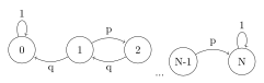
It is easy to see that \(0\) and \(N\) are recurrent states and the remaining states are transient.

Stationary distribution

Definition C.8.

For a DTMC with transition probability matrix \(P\), the vector \(\pi=(\pi_i, i\in \X)\) is called a stationary distribution if

1. \(\pi_i\ge 0,\, \forall i\) and \(\sum_{i} \pi_i=1\).

2. \(\pi=\pi P\).

The first condition above implies \(\pi\) is a distribution, while the second condition relates to stationarity. In particular, if the initial distribution of the DTMC is \(X_0\sim \pi\), then the distribution of the state \(X_n\) (at instant \(n\)) is:

\[ \pi P^n = \pi P P^{n-1}=\pi P^{n-1} = \ldots = \pi. \]

The main result concerning the existence of stationary distribution is given below.

Theorem C.1.

Consider an irreducible DTMC \(\{X_n\}\). Then,

1. There exists a stationary distribution if and only if some state in the DTMC is positive recurrent.

2. If there exists a stationary distribution \(\pi\), then every state is positive recurrent, and

   \[ \pi_i=\frac{1}{m_i}, \textrm{ where } m_i=\E[T_i\mid X_0=i], \]

   and \(T_i=\min\{n\ge 1\mid X_n=i\}\).

3. \(\pi\) is unique.

Example C.10.

For the two state DTMC in Example C.1 with \(\alpha + \beta < 2\), the set of equations for finding the stationary distribution are as follows:

\[ \begin{align*} &\pi_0=\alpha \pi_0 + (1-\beta)\pi_1, \\ &\pi_1= (1-\alpha)\pi_0 + \beta \pi_1, \\ &\pi_0+\pi_1=1. \end{align*} \]

Solving, we obtain \(\pi_0=\frac{1-\beta}{1-\alpha-\beta}\), and \(\pi_1=\frac{1-\alpha}{1-\alpha-\beta}\). This coincides with the limit of \(P^n\) as well as \(M^n/(n+1)\), as discussed in Example C.6. We discuss convergence to stationary distribution next.

Periodicity

We require the notion of period associated with a recurrent state before we understand convergence to stationary distribution. We define this notion below.

Definition C.9.

Let \(\tilde T_i = \min\{n > 0: X_n = i\}, i \in \X\). Let \(i\) be a recurrent state and \(d\) the largest positive integer such that

\[ \sum_{k=1}^{\infty} P(\tilde T_i = kd) = 1. \]

If \(d = 1\), then state \(i\) is aperiodic. On the other hand, if \(d > 1\), then state \(i\) is said to be periodic with period \(d\).

Equivalently, if \(i\) is a recurrent state with period \(d\), then \(P_{i,i}^{(n)} = 0\) for all n that are not positive integer multiples of \(d\).

Remark C.1.

Periodicity is a class property, i.e., if \(i \leftrightarrow j\), then \(i, j\) have the same period.

As an example, consider a symmetric random walk, i.e., \(P_{i,i+1}=P_{i,i-1}=1/2\) for all \(i\). In this case, it is easy to see that the period of state \(0\) is two and by using the fact that the chain is irreducible, all states have period \(2\).

Convergence to stationary distribution

In Example C.6, we observed that \(P^n\) and \(\frac{M^n}{n+1}\) both converged, whereas in Example C.7, \(P^n\) did not converge. The distinguishing feature between these two examples is that one of the is aperiodic and the other not. The result below formalizes convergence to stationary distribution for aperiodic chains.

Theorem C.2.

Let \(\{X_n\}\) be an irreducible, recurrent, aperiodic DTMC. Then, for any \(i,j\in \X\), we have

\[ P^{(n)}_{i,j}\rightarrow \pi_j \textrm{ as } n\rightarrow\infty, \]

where \(\pi\) is the (unique) stationary distribution.

A easy counterexample that emphasizes the need for aperiodicity to ensure \(P^{(n)}\) converges is a two state DTMC with \(P=\begin{bmatrix} 0&1\\1&0 \end{bmatrix}.\)

For periodic DTMCs, one can claim convergence to stationary distribution in the so-called “Cesaro sense”. We formalize this statement next.

Let \(\tilde V_n(j)= \sum_{m=1}^n \indic{X_m=j}\) denote the occupancy measure for state \(j\). We are interested in knowing if the time-averaged occupancy, i.e., \(\frac{1}{n} \tilde V_n(j)\), converges to the stationary distribution as \(n\rightarrow\infty\) for an irreducible recurrent DTMC. Such a law of large numbers type result is stated next.

Theorem C.3.

Let \(\{X_n\}\) be an irreducible, recurrent DTMC. Then, for any \(j\in \X\), we have the following for any start state:

\[ \begin{align*} \frac{1}{n} \tilde V_n(j) \rightarrow \frac{\indic{T_j<\infty}}{m_j} \textrm{ a.s. as } n\rightarrow\infty. \tag{C.3} \end{align*} \]

A few remarks are in order.

Remark C.2.

From the result above, we have \(\frac{1}{n} \tilde V_n(j)\) converges to \(\pi_j=\frac{1}{m_j}\) if \(j\) is positive recurrent, and to \(0\) otherwise. The latter case includes null recurrent states, and a similar claim can be shown for transient states as well.

Remark C.3.

Notice that

\[ \begin{align*} \E\left[\frac{1}{n} \tilde V_n(j)\mid X_0=i\right]= \frac{1}{n} \sum_{m=1}^n \E\left[ \indic{X_m=j} \mid X_0=i\right] =\frac{1}{n} \sum_{m=1}^n P^{(m)}(i,j), \end{align*} \]

and

\[ \E\left[\frac{\indic{T_j<\infty}}{m_j}\mid X_0=i\right]= \frac{\Prob{T_j<\infty \mid X_0=i}}{m_j}. \]

Thus,

\[ \frac{1}{n} \sum_{m=1}^n P^{(m)}(i,j) \rightarrow \frac{\Prob{T_j<\infty \mid X_0=i}}{m_j} \textrm{ a.s. as } n \rightarrow\infty. \]

The limit on the RHS above is zero for null recurrent states \(j\) and likewise positive for positive recurrent \(j\).

Remark C.4.

For a transient state \(j\), \(\sum_{m=1}^{\infty} P^{(m)}(i,j) < \infty\). Hence,

\[ \begin{align*} \E\left[\frac{1}{n} \tilde V_n(j)\mid X_0=i\right] =\frac{1}{n} \sum_{m=1}^n P^{(m)}(i,j) \\ \rightarrow 0 \textrm{ a.s. as } n \rightarrow\infty. \end{align*} \]

C.4 Bibliographic remarks

There are several excellent textbooks for Markov chains, for instance, (Levin and Peres 2017; Meyn and Tweedie 2012; Grimmett and Stirzaker 2020; Norris 1998; Gallager 2013; Kulkarni 2016). Our treatment is based on a combination of (Kulkarni 2016) and (Grimmett and Stirzaker 2020).

C.5 Exercises

Exercise 1.

Let \(\{X_n,n\ge 0\}\) be a DTMC. Then,

\[ \Prob{X_0 =i,X_2 =k\mid X_1 = j}=\Prob{X_0 =i\mid X_1 = j}\Prob{X_2 =k\mid X_1 = j}. \]

Exercise 2.

Suppose \(\{X_{n}, n \geq 0\}\) and \(\{Y_{n}, n \geq 0\}\) are two independent DTMCs with state-space \(S = \{0, 1, 2,\ldots\}.\) Prove or give a counterexample to the following statements:

1. \(\{X_{n} + Y_{n}, n \geq 0 \}\) is a DTMC.

2. \(\{(X_{n}, Y_{n}), n \geq 0\}\) is a DTMC.

Exercise 3.

Consider a DTMC on state space \(\{1,2,3,4,5\}\), with the following transition probability matrix:

\[ P =\begin{bmatrix} 0 &0.5 &0.5&0&0\\ 0 &0 &0 & 0.5&0.5\\ 0 &0 &0 & 0.5&0.5\\ 1 &0 &0 & 0&0\\ 0.5 &0 &0 & 0&0.5 \end{bmatrix}. \]

Answer the following:

1. Is the DTMC irreducible? Aperiodic?

2. Let \(T= \min\{n\ge 0 \mid X_n=4\}\). Compute \(\Prob{T<\infty\mid X_0=1}\).

Exercise 4.

Consider a random walk with \(p_{0,0} = p_{N,N}=1\), and \(p_{i,i+1}=p=1-p_{i,i-1}\) for \(1\le i \le N-1\). Let \(T\) be the first passage time to either \(0\) or \(N\), i.e., \(T= \min\{n\ge 0 \mid X_n=0 \textrm{ or } N\}\).

Answer the following:

1. In the case where \(p\ne \frac{1}{2}\), show that

   \[ \EE{T\mid X_0=i} = \dfrac{i}{q-p} - \left(\dfrac{N}{q-p}\right) \left(\dfrac{1- \left(\frac{q}{p}\right)^i}{1- \left(\frac{q}{p}\right)^N}\right). \]

2. Compute \(\EE{T\mid X_0=i}\) when \(p=\frac{1}{2}\).

Exercise 5.

For each of the following statements, either provide a proof or disprove by exhibiting a counterexample.

1. A finite DTMC has at least one closed communicating class.

2. If a DTMC is periodic, then it is not positive recurrent.

3. Every finite DTMC possesses a stationary distribution.

4. Consider a finite DTMC with state space \(\{0,1,\ldots,K\}\). Let \(T=\sup\{n\ge0\mid X_n =0\}\). Then, \(T\) is a stopping time.

5. In a DTMC, a state \(i\) is transient only if there exists a state \(j\) such that \(j\) is accessible from \(i\), but \(i\) is not accessible from \(j\).

6. A finite irreducible DTMC is aperiodic if and only if \(\exists n >0\) such that \(p_{i,j}^{(n)} >0\), \(\forall i,j\).

Exercise 6.

Consider a DTMC space with state space \(\{1,2,\ldots,N\}\) with the following \(N \times N\) transition probability matrix

\[ \left[ \begin{array}{ccccccccccccccccccc} q & p & 0 & 0 & 0 & . & . & . & . & . & 0 & 0 & 0 \\ q & 0 & p & 0 & 0 & . & . & . & . & . & 0 & 0 & 0 \\ 0 & q & 0 & p & 0 & . & . & . & . & . & 0 & 0 & 0 \\ .\\ .\\ .\\ 0 & . & . & . & 0 & 0 & q & 0 & p & 0 & . & . & 0 .\\ .\\ .\\ 0 & 0 & 0 & 0 & . & . & . & . & . & 0 & q & 0 & p \\ 0 & 0 & 0 & 0 & . & . & . & . & . & 0 & 0 & q & p \\ \end{array} \right] \]

Answer the following:

1. Is the DTMC irreducible ?

2. Is the DTMC periodic ?

3. Does the DTMC have stationary distribution. If yes, provide the same.

Exercise 7.

Consider a DTMC on \(\{0,1,2,\ldots\}\) with \(p_{0,0} = 1\), and \(p_{i,i-1}=q=1-p_{i,i}\) for \(i\ge 1\).

Answer the following:

1. Find \(\Prob{X_n=0, X_m \ne 0, \textrm{for } 0<m<n \mid X_0=i}\) for \(i\ge 1\).

2. What is the expected value of the distribution from the part above?

Exercise 8.

Consider a random walk with \(p_{i,i+1}=p\), and \(p_{i,i-1} = q\), for \(-\infty<i<\infty\). Here \(0<p<1\) and \(p+q=1\).

Answer the following, assuming that the random walk starts at the origin:

1. Find the probability that the random walk hits state \(i\) before hitting state \(-j\), where \((i,j>0)\).

2. Show that the expected number of visits to the state \(i\) before hitting state \(0\) is \(\left(\frac{p}{q}\right)^i\) , when \(p<q\).

3. What would the expected value from the part above be when \(p=q\)?

Exercise 9.

For the DTMCs with transition probability matrices listed below, identify the communicating classes, and determine their transience/recurrence. Further, for each \(i,j\) in the state space, find \(\lim\limits_{n\rightarrow\infty} p_{i,j}^{(n)}\).

1. \(P =\begin{bmatrix} 0 &0.4 &0.6\\ 0.1 &0 &0.9\\ 0.3 &0.7 &0 \end{bmatrix}\).

2. \(P =\begin{bmatrix} 0 &0 &0&1\\ 0 &0 &0 & 1\\ 0.3 &0.7 &0&0\\ 0&0&1&0 \end{bmatrix}\).

Exercise 10.

Suppose there are two urns, say \(1\) and \(2\). Each urn has \(r\) balls. Among the \(2r\) balls, \(b\le r\) balls are black, and the remaining \(2r - b\) are white. At each trial, one ball is picked uniformly at random from each urn, and they are interchanged.

Answer the following:

1. Model this problem as a DTMC with the state as the number of white balls in urn \(1\). Specify the state space and transition probabilities. Is the DTMC irreducible? Aperiodic?

2. Compute the stationary distribution.

Gallager, Robert G. 2013. Stochastic Processes: Theory for Applications. Cambridge University Press.

Grimmett, Geoffrey, and David Stirzaker. 2020. Probability and Random Processes. Oxford university press.

Kulkarni, Vidyadhar G. 2016. Modeling and Analysis of Stochastic Systems. Chapman; Hall/CRC.

Levin, David A, and Yuval Peres. 2017. Markov Chains and Mixing Times. Vol. 107. American Mathematical Soc.

Meyn, Sean P, and Richard L Tweedie. 2012. Markov Chains and Stochastic Stability. Springer Science & Business Media.

Norris, James R. 1998. Markov Chains. 2. Cambridge university press.